

How can the Normal Distribution arise out of a completely symmetric set-up? The so-called Central Limit Theorem (CLT) is a fascinating example that demonstrates such behaviour. If you want to get some intuition on what lies at the core of many statistical tests, read on!
The Central Limit Theorem (CLT) states:
When a large number of samples of size n of independent and identically distributed (i.i.d.) random variables are drawn from any population with a finite mean and finite variance, the distribution of the sum (or the average = scaled sum) of these samples will tend to be normally distributed, regardless of the original population distribution. This is what gives the Normal Distribution (= bell curve or Gaussian distribution) its special status.
What are i.i.d. random variables? A few years ago I gave the following explanation on Cross Validated:
A good example is a succession of throws of a fair coin: The coin has no memory, so all the throws are “independent”. And every throw is 50:50 (heads:tails), so the coin is and stays fair – the distribution from which every throw is drawn, so to speak, is and stays the same: “identically distributed”.
As an example, let us start with a simple fair die, which gives us a perfectly symmetric uniform (discrete) distribution form 1 to 6:
plot_hist <- function(x) {
  plot(sort(x), sequence(table(x)), xlab = "", ylab = "")
}

X <- 1:6 # one die
plot_hist(X)
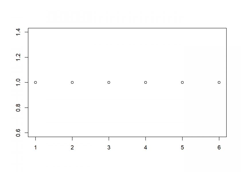
Or as a frequency table:
table(X)
## X
## 1 2 3 4 5 6
## 1 1 1 1 1 1
Now, we either throw this die twice and add the dots or we take two dice, again adding their dots. The range obviously lies between 2 and 12, but not all of those outcomes are created equal:
X2 <- rowSums(expand.grid(1:6, 1:6))
plot_hist(X2)
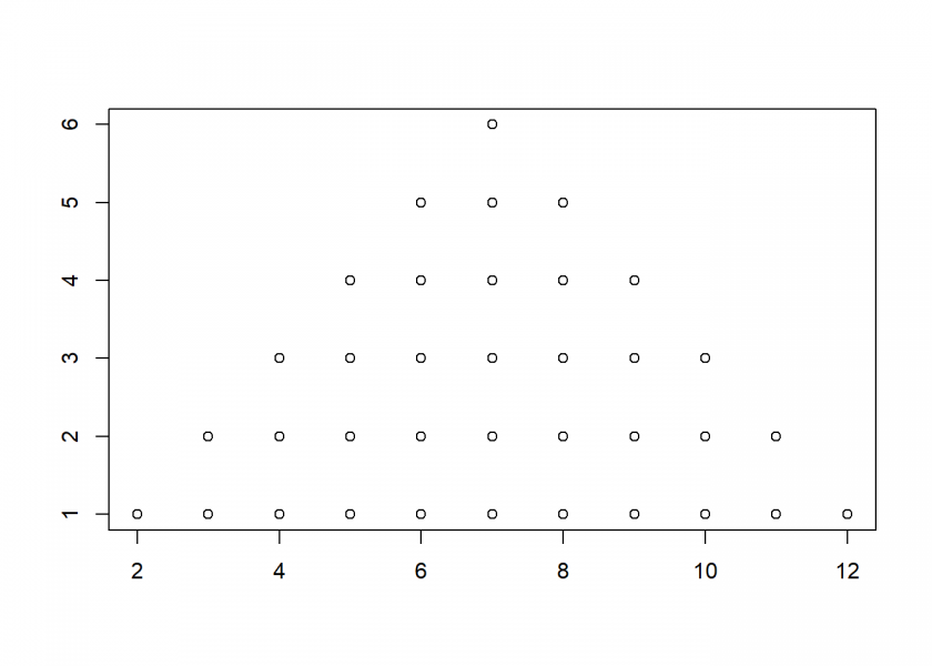
Again as a frequency table:
table(X2)
## X2
##  2  3  4  5  6  7  8  9 10 11 12
##  1  2  3  4  5  6  5  4  3  2  1
We can see that 2 and 12 only have one possibility of happening (1+1 and 6+6), whereas 7 has six different combinations (1+6, 2+5, 3+4, 4+3, 5+2 and 6+1).
Here we are at the center of the symmetry-break: we have two perfectly symmetric entities and by combining them we get a triangle-like structure. Why? Basically this is what is happening:
Mathematically this is called a convolution: by summing all possible combinations you are sliding the original uniform distribution over itself. This naturally produces less overlap (= sum) at the edges and maximal overlap at the center!
You can continue in this manner, taking the sum of three dice…
X3 <- rowSums(expand.grid(1:6, 1:6, 1:6))
plot_hist(X3)
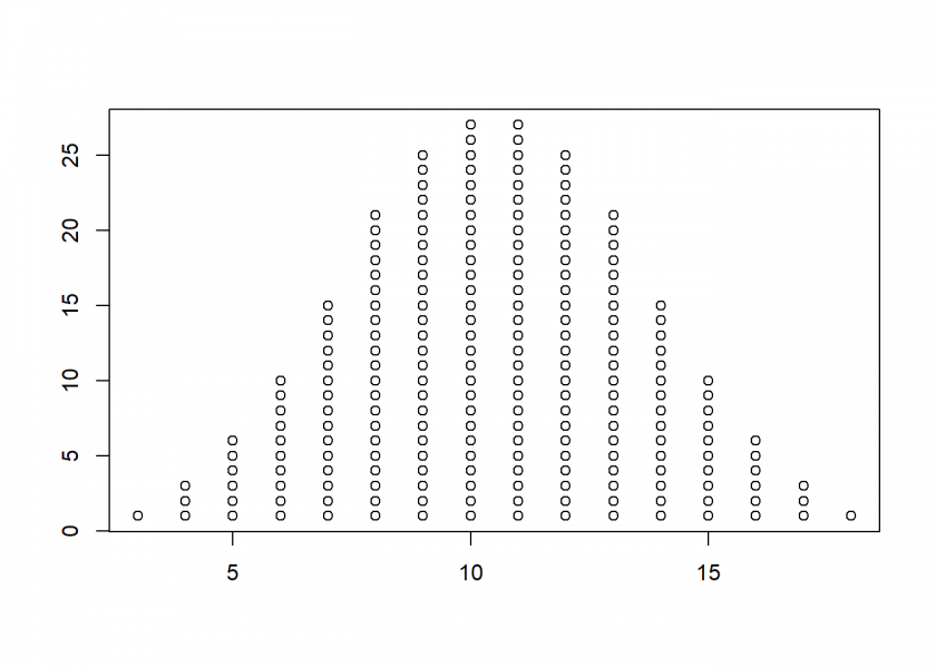
…and four dice, superimposing a fitted normal distribution:
X4 <- rowSums(expand.grid(1:6, 1:6, 1:6, 1:6))
plot_hist(X4)
curve(dnorm(x, mean = mean(X4), sd = sd(X4)) * length(X4), add = TRUE)
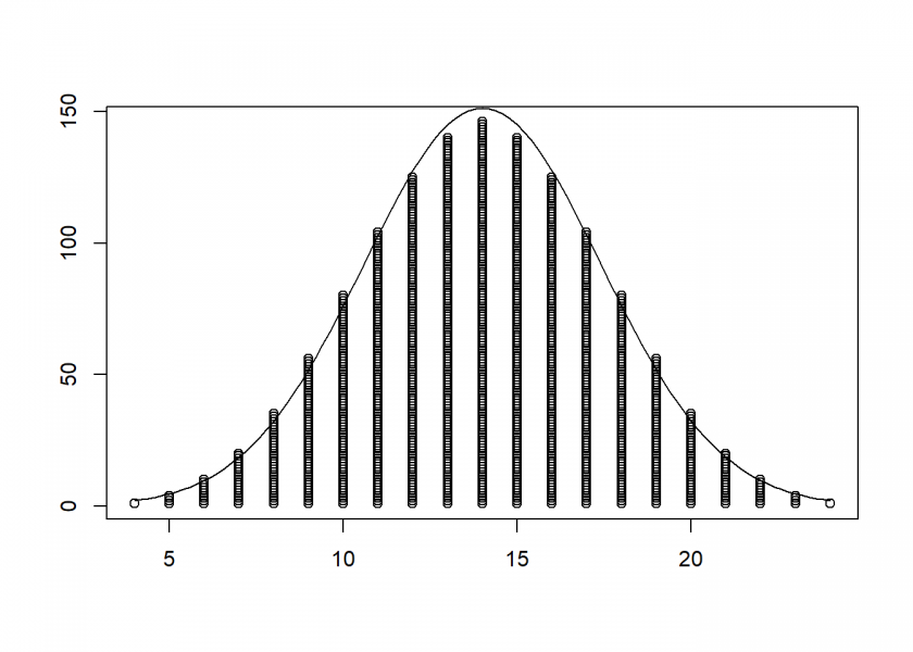
You can see that the resulting structure resembles the normal distribution more and more. Seen this way the Normal Distribution is the honed triangle from above!
Because there are many processes in real life that act additively (like e.g. growth processes) the Normal Distribution holds a special place in many real-world phenomena (e.g. heights). This is the reason why it constitutes the basis for many statistical tests in inferential (= inductive) statistics (see also From Coin Tosses to p-Hacking: Make Statistics Significant Again!).
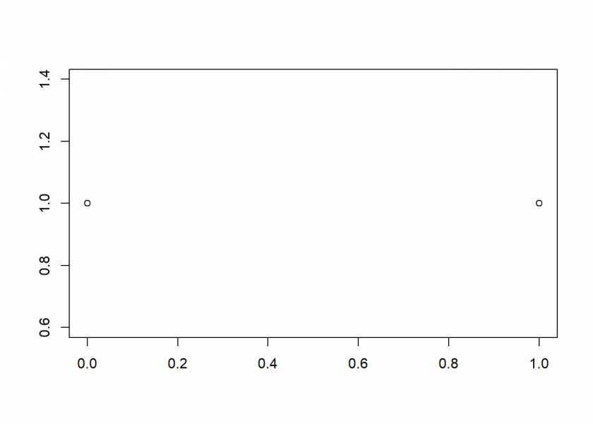
The go even more minimalistic, we can even see this symmetry-break with said coin tosses:
X <- 0:1 # one coin
plot_hist(X)
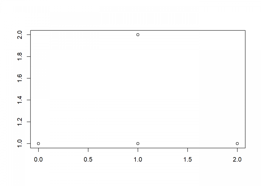
X2 <- rowSums(expand.grid(0:1, 0:1))
plot_hist(X2)
To answer our starting question: in the end, it is the process, or more exactly, the mathematical operation that we use (sliding over the outcomes of our random experiments) which gives us a honed version of a triangle: the Normal Distribution!
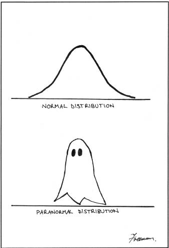
Yet the derivation of the Paranormal Distribution remains a mystery… 😉
Gaussian distribution (family) owes its prominence to finite variance, for it is the only one with that property in the greater family of alpha-stable distributions. But some additive processes in nature or human activity are described by other stable distributions, and there is a generalized form of CLT to account for their emergence. This is, as usual, neatly summarized in Wikipedia, so I refer the interested to there.
Thank you, Lauri, this is highly appreciated!
Packages
Stable,StableDistandStableEstimprovide functionality related to alpha-stable distributions in R, so maybe you’ll take them for a test drive in future posts.Are you perhaps interested in writing a guest post?
I’m honoured by your suggestion. I’ve used the packages previously while working with financial markets data. (Mandelbrot introduced the distributions into finance in 1963, though received mostly academic interest until Nassim Taleb brought “fat tails” into everyone’s attention. Taleb gives full credit to Mandelbrot.) I tend to be lazy with demonstrations, always picking the lowest-hanging fruit. So I feel that I should write about the mathematical foundation (can’t be lazy with that). You could follow up with R demonstrations. I’ll get back to this.
I was fortunate enough to meet both Mandelbrot and Taleb: I met Mandelbrot at the Frankfurt Book Fair where he received a prize from the Financial Times for his book “The misbehaviour of markets”. For Taleb: I once had a two-days seminar on trading and quant finance which was collaboratively held by Paul Wilmott and Nassim Taleb in London. All three characters are (were) fascinating in their own way!
Your suggestion sounds great, looking forward to hearing back from you!
The animated graph you had of the convolution of two uniform distributions reminded me of a very nifty attribute of uniform distributions, namely, their variance is (1/12)*(u – l)^2, where u=upper bound and l=lower bound. This means that the sum of 12 iid uniform distributions will have a variance of (u – l)^2 or standard deviation of (u – l). The mean of the sum will be 12*(u+l)/2 = 6*(u – l). What this leads to is that we can specify a Normal distribution simulation as
Normal(m, sd) ~ Sum( {Uniform(n, (m-6*sd)/12, (m+6*sd)/12)}/j, j)
where n is the number of simulation trials, and j is an index on 1:12 across which each uniform is simulated. So, if you find yourself in need of simulating a Normal distribution without a modern simulation engine that uses a closed form solution for the cumulative probability distribution of a Normal, the convolution of 12 uniform distributions provides an excellent approximation (unless you want the possibility of samples to occur from the extreme tails of the Normal).
Here is some sample code to demonstrate this:
That is amazing! Your contributions are always highly appreciated!
Thank you so much!
Here’s a slightly simpler way to run the Normal approximation:
This slight modification to the last approach is based on simulating the unit Normal and that m + k*Normal(0, s) = m + Normal(0, k*s).
Good day. I have been enjoying the nice explanations in this post. Thank you for your clear and interesting explanations. I have a question. How can I subscribe to this post?
That is very nice of you, Jose, thank you!
There are several possibilities:
– Subscribe to the RSS feed with an RSS reader: https://blog.ephorie.de/feed
– Follow my LinkedIn activities: https://www.linkedin.com/in/vonjd/
– Follow my twitter feed: @ephorie
I am always open to feedback (also critical! Always eager to learn!) – Thank you again
Thank you so much.
Best wishes