

Election polls play a crucial role in predicting the outcome of elections and shaping public opinion. However, it’s important to understand that the results of any single poll should be taken with a grain of salt.
Many polls only ask about 1,000 people about their political preferences, which is quite small in comparison to the often millions of voters. So, how reliable are those results? Or in other words, how confident can we be in the results? To understand some of these intricacies, read on!
You can also watch the video for this post (in German):
In this blog post, we will explore what confidence intervals are, why they are important in election polling, and how to calculate them using an example with three parties, one with 50% of the vote, one with 25% and one with 5%. We’ll also use R code to simulate the margin of error for each party and demonstrate the difference in uncertainty between the three. By the end of this post, you’ll have a better understanding of how to interpret election polls and the limitations of political forecasting.
Confidence intervals have a rather unintuitive technical definition, but the general idea is that they are a way to express the uncertainty surrounding an estimate. For example, in the context of election polls, a poll might estimate that a certain party will receive x% of the vote, but with a margin of error of ±y%. This means, that if the poll were repeated many times, and a confidence interval calculated from each sample, we would expect that 95% (i.e. the confidence level) of these intervals would contain the party’s true support.
So, intuitively speaking, the confidence interval gives us a range of values that we are fairly confident contains the true value of what we are trying to estimate. In this case, the true level of support for a party. The wider the confidence interval, the less certain we are about the estimate. The narrower the confidence interval, the more certain we are.
It’s important to note that a confidence interval does not guarantee that the true value will be within the range, just that 95% of all confidence intervals that were calculated this way will cover the true value.
Another kind of interval, which gives the probability that the estimated parameter is covered with, for example, a 95% probability, is a Bayesian credible interval. Interestingly enough, while their interpretation is quite different (and admittedly more intuitive), in our specific case, the results are not too far apart from each other. Therefore, the more intuitive, but commonly misinterpreted, view of frequentist confidence intervals wouldn’t be too far off in this instance.
Now, for another important point: the relative margin of error (relative with respect to the support of the party) would increase if you’re estimating support for a party with 5% of the vote compared to a party with 50% of the vote. This is because the margin of error is affected by the sample size and the level of variability in the data. When the sample size is small or the level of variability is high, the relative margin of error will be larger.
In the case of a party with 5% of the vote, the sample size of voters supporting that party will be smaller, leading to a higher level of variability. This, in turn, will result in a larger relative margin of error, meaning the range of possible values for the estimate of the party’s support will be wider.
To put it another way, it’s easier to estimate the level of support for a party with 50% of the vote because there are many more voters to sample from and the results are less variable. On the other hand, it’s harder to estimate the level of support for a party with 5% of the vote because there are fewer voters to sample from and the results are more variable.
So, if all else is equal (same level of confidence, same sample size, etc.), the relative margin of error would be larger for a party with 5% of the vote compared to a party with 50% of the vote.
Let us demonstrate this effect with R by simulating 10,000 sample polls with 1,000 respondents for each party:
set.seed(123) # for reproducibility

# poll_sim function
poll_sim <- function(p = 0.25, n = 1000, n_sim = 10000, conf_int = 0.95) {

  # Z-score for the given confidence level
  z_score <- qnorm(1 - (1 - conf_int) / 2)

  # Store the results of the simulations
  results <- rep(NA, n_sim)

  # Run the simulations
  for (i in 1:n_sim) {
    # Generate a sample of binary responses (0 or 1)
    sample <- rbinom(n, size = 1, prob = p)

    # Calculate the proportion of 1's (i.e., the estimate of p)
    results[i] <- mean(sample)
  }

  # Calculate the margin of error
  moe <- z_score * sqrt(p * (1 - p) / n)

  # Plot the results
  hist(results, main = paste0("Party with Proportion ", p * 100, "%"), xlab = "Estimated Proportion", col = "blue")
  abline(v = p, col = "red", lwd = 3)
  abline(v = p + moe, col = "green", lty = 2, lwd = 3)
  abline(v = p - moe, col = "green", lty = 2, lwd = 3)

  # Show margin of error
  cat("Absolute Margin of Error:", round(moe, 3), "\n")
  cat("Confi. Int. from", round(p - moe, 3), "to", round(p + moe, 3), "\n")
  cat("Relative Margin of Error:", round(moe / p, 3), "\n")
}

# Parameters
p1 <- 0.5  # True proportion of votes for party 1 (50%)
p2 <- 0.25 # True proportion of votes for party 2 (25%)
p3 <- 0.05 # True proportion of votes for party 3 (5%)
n <- 1000  # Sample size

# Number of simulations
n_sim <- 10000

# Run the simulations
poll_sim(p1)
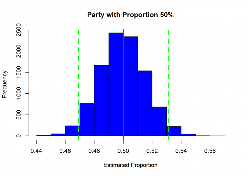
## Absolute Margin of Error: 0.031
## Confi. Int. from 0.469 to 0.531
## Relative Margin of Error: 0.062
So, in this case, the absolute margin of error is indeed ±3%.
poll_sim(p2)
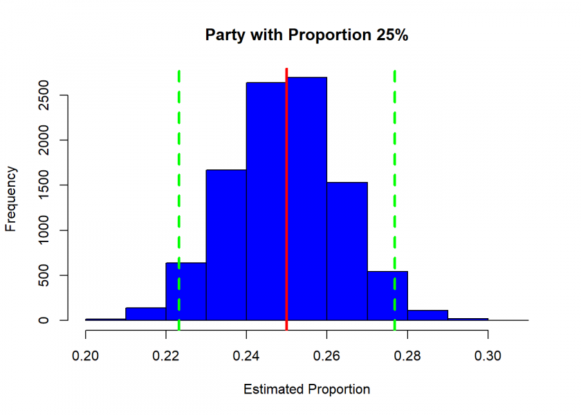
## Absolute Margin of Error: 0.027
## Confi. Int. from 0.223 to 0.277
## Relative Margin of Error: 0.107
In the case of a party with a true proportion of 25% the relative margin of error becomes over 10%!
poll_sim(p3)
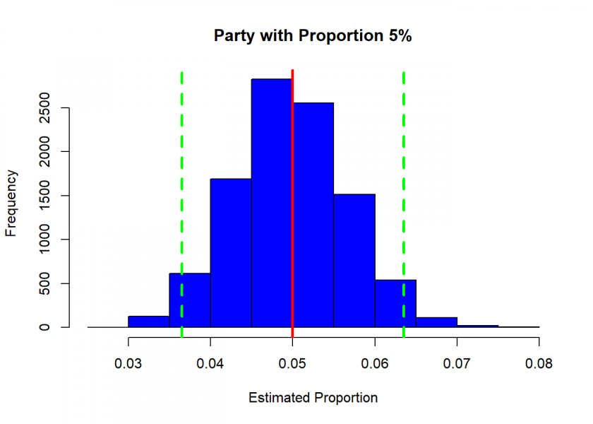
## Absolute Margin of Error: 0.014
## Confi. Int. from 0.036 to 0.064
## Relative Margin of Error: 0.27
So, while the absolute margin of error is much smaller in this case (about half of the first case), the relative level of uncertainty is much bigger (nearly 30%)!
In conclusion, confidence intervals are a crucial tool in understanding the uncertainty of election polling results. Our simulation of the margin of error for three parties highlights the importance of considering the level of uncertainty when interpreting election polls. We hope this post has provided you with a clearer understanding of confidence intervals and how to apply them to election polling.