

R is a powerful programming language and environment for statistical computing and graphics. In this post, we will provide a quick introduction to R using the famous iris dataset.
We will cover loading data, exploring the dataset, basic data manipulation, and plotting. By the end, you should have a good understanding of how to get started with R, so read on!
This is the introduction that I wished I had back when I started analyzing data! Disclosure: part of the post and code were written with the assistance of ChatGPT-4, the concept and ideas herein are my own.
You can also watch the video for this post (in German):
Getting Started
First, download and install R from the Comprehensive R Archive Network (CRAN): https://cran.r-project.org/
Next, download and install RStudio, an integrated development environment (IDE) for R: https://posit.co/download/rstudio-desktop/
Ok, and now see for yourself how easy it is to analyze data with R! We will use the equivalent of “Hello World” for data science, the famous iris dataset. Of course, you can also easily load your own data into R: just click on “Import Dataset” in the “Environment” tab in the upper right window of RStudio and follow the steps from there!
The iris dataset is a classic and widely used dataset in the field of data science and machine learning. The dataset consists of 150 samples from three species of iris flowers: Iris setosa, Iris versicolor, and Iris virginica. Each sample contains four features, which are the lengths and widths of the sepals and petals (in centimeters). The dataset has become a popular choice for testing and demonstrating various data analysis and machine learning techniques due to its simplicity and well-defined structure. The iris dataset comes pre-loaded in R, so no need to import any external files.
Exploring the Dataset
To get an overview of the dataset, use the head() and summary() functions:
# Display the first 6 rows of the dataset
head(iris)
##   Sepal.Length Sepal.Width Petal.Length Petal.Width Species
## 1          5.1         3.5          1.4         0.2  setosa
## 2          4.9         3.0          1.4         0.2  setosa
## 3          4.7         3.2          1.3         0.2  setosa
## 4          4.6         3.1          1.5         0.2  setosa
## 5          5.0         3.6          1.4         0.2  setosa
## 6          5.4         3.9          1.7         0.4  setosa

# Get summary statistics of the dataset
summary(iris)
##   Sepal.Length    Sepal.Width     Petal.Length    Petal.Width
##  Min.   :4.300   Min.   :2.000   Min.   :1.000   Min.   :0.100
##  1st Qu.:5.100   1st Qu.:2.800   1st Qu.:1.600   1st Qu.:0.300
##  Median :5.800   Median :3.000   Median :4.350   Median :1.300
##  Mean   :5.843   Mean   :3.057   Mean   :3.758   Mean   :1.199
##  3rd Qu.:6.400   3rd Qu.:3.300   3rd Qu.:5.100   3rd Qu.:1.800
##  Max.   :7.900   Max.   :4.400   Max.   :6.900   Max.   :2.500
##        Species
##  setosa    :50
##  versicolor:50
##  virginica :50
The summary() function in R provides a quick overview of the main statistical measures for numerical data. Here are short descriptions of each measure:
- Minimum (Min.): The smallest value in the dataset.
- 1st Quartile (1st Qu.): The value that separates the lowest 25% of the data from the remaining 75%; also known as the 25th percentile.
- Median (2nd Qu.): The middle value that separates the lower and upper halves of the data; also known as the 50th percentile.
- Mean: The arithmetic average of the data values, calculated by adding up all the values and dividing by the total number of values.
- 3rd Quartile (3rd Qu.): The value that separates the lowest 75% of the data from the highest 25%; also known as the 75th percentile.
- Maximum (Max.): The largest value in the dataset.
These statistical measures give you a quick snapshot of the central tendency, dispersion, and overall distribution of your numerical data.
Data Manipulation
a) Subsetting the dataset
To select specific columns in the dataset, use the $ operator or the [] brackets:
# Select the Petal.Width column
iris$Petal.Width
##   [1] 0.2 0.2 0.2 0.2 0.2 0.4 0.3 0.2 0.2 0.1 0.2 0.2 0.1 0.1 0.2 0.4 0.4 0.3
##  [19] 0.3 0.3 0.2 0.4 0.2 0.5 0.2 0.2 0.4 0.2 0.2 0.2 0.2 0.4 0.1 0.2 0.2 0.2
##  [37] 0.2 0.1 0.2 0.2 0.3 0.3 0.2 0.6 0.4 0.3 0.2 0.2 0.2 0.2 1.4 1.5 1.5 1.3
##  [55] 1.5 1.3 1.6 1.0 1.3 1.4 1.0 1.5 1.0 1.4 1.3 1.4 1.5 1.0 1.5 1.1 1.8 1.3
##  [73] 1.5 1.2 1.3 1.4 1.4 1.7 1.5 1.0 1.1 1.0 1.2 1.6 1.5 1.6 1.5 1.3 1.3 1.3
##  [91] 1.2 1.4 1.2 1.0 1.3 1.2 1.3 1.3 1.1 1.3 2.5 1.9 2.1 1.8 2.2 2.1 1.7 1.8
## [109] 1.8 2.5 2.0 1.9 2.1 2.0 2.4 2.3 1.8 2.2 2.3 1.5 2.3 2.0 2.0 1.8 2.1 1.8
## [127] 1.8 1.8 2.1 1.6 1.9 2.0 2.2 1.5 1.4 2.3 2.4 1.8 1.8 2.1 2.4 2.3 1.9 2.3
## [145] 2.5 2.3 1.9 2.0 2.3 1.8

# Select the first three columns (the first part before the comma is for selecting the rows, the second is for the columns - if left free, nothing is filtered)
iris[ , 1:3]
##     Sepal.Length Sepal.Width Petal.Length
## 1            5.1         3.5          1.4
## 2            4.9         3.0          1.4
## 3            4.7         3.2          1.3
## 4            4.6         3.1          1.5
## 5            5.0         3.6          1.4
## 6            5.4         3.9          1.7
## 7            4.6         3.4          1.4
## 8            5.0         3.4          1.5
## 9            4.4         2.9          1.4
## 10           4.9         3.1          1.5
## 11           5.4         3.7          1.5
## 12           4.8         3.4          1.6
## 13           4.8         3.0          1.4
## 14           4.3         3.0          1.1
## 15           5.8         4.0          1.2
## 16           5.7         4.4          1.5
## 17           5.4         3.9          1.3
## 18           5.1         3.5          1.4
## 19           5.7         3.8          1.7
## 20           5.1         3.8          1.5
## 21           5.4         3.4          1.7
## 22           5.1         3.7          1.5
## 23           4.6         3.6          1.0
## 24           5.1         3.3          1.7
## 25           4.8         3.4          1.9
## 26           5.0         3.0          1.6
## 27           5.0         3.4          1.6
## 28           5.2         3.5          1.5
## 29           5.2         3.4          1.4
## 30           4.7         3.2          1.6
## 31           4.8         3.1          1.6
## 32           5.4         3.4          1.5
## 33           5.2         4.1          1.5
## 34           5.5         4.2          1.4
## 35           4.9         3.1          1.5
## 36           5.0         3.2          1.2
## 37           5.5         3.5          1.3
## 38           4.9         3.6          1.4
## 39           4.4         3.0          1.3
## 40           5.1         3.4          1.5
## 41           5.0         3.5          1.3
## 42           4.5         2.3          1.3
## 43           4.4         3.2          1.3
## 44           5.0         3.5          1.6
## 45           5.1         3.8          1.9
## 46           4.8         3.0          1.4
## 47           5.1         3.8          1.6
## 48           4.6         3.2          1.4
## 49           5.3         3.7          1.5
## 50           5.0         3.3          1.4
## 51           7.0         3.2          4.7
## 52           6.4         3.2          4.5
## 53           6.9         3.1          4.9
## 54           5.5         2.3          4.0
## 55           6.5         2.8          4.6
## 56           5.7         2.8          4.5
## 57           6.3         3.3          4.7
## 58           4.9         2.4          3.3
## 59           6.6         2.9          4.6
## 60           5.2         2.7          3.9
## 61           5.0         2.0          3.5
## 62           5.9         3.0          4.2
## 63           6.0         2.2          4.0
## 64           6.1         2.9          4.7
## 65           5.6         2.9          3.6
## 66           6.7         3.1          4.4
## 67           5.6         3.0          4.5
## 68           5.8         2.7          4.1
## 69           6.2         2.2          4.5
## 70           5.6         2.5          3.9
## 71           5.9         3.2          4.8
## 72           6.1         2.8          4.0
## 73           6.3         2.5          4.9
## 74           6.1         2.8          4.7
## 75           6.4         2.9          4.3
## 76           6.6         3.0          4.4
## 77           6.8         2.8          4.8
## 78           6.7         3.0          5.0
## 79           6.0         2.9          4.5
## 80           5.7         2.6          3.5
## 81           5.5         2.4          3.8
## 82           5.5         2.4          3.7
## 83           5.8         2.7          3.9
## 84           6.0         2.7          5.1
## 85           5.4         3.0          4.5
## 86           6.0         3.4          4.5
## 87           6.7         3.1          4.7
## 88           6.3         2.3          4.4
## 89           5.6         3.0          4.1
## 90           5.5         2.5          4.0
## 91           5.5         2.6          4.4
## 92           6.1         3.0          4.6
## 93           5.8         2.6          4.0
## 94           5.0         2.3          3.3
## 95           5.6         2.7          4.2
## 96           5.7         3.0          4.2
## 97           5.7         2.9          4.2
## 98           6.2         2.9          4.3
## 99           5.1         2.5          3.0
## 100          5.7         2.8          4.1
## 101          6.3         3.3          6.0
## 102          5.8         2.7          5.1
## 103          7.1         3.0          5.9
## 104          6.3         2.9          5.6
## 105          6.5         3.0          5.8
## 106          7.6         3.0          6.6
## 107          4.9         2.5          4.5
## 108          7.3         2.9          6.3
## 109          6.7         2.5          5.8
## 110          7.2         3.6          6.1
## 111          6.5         3.2          5.1
## 112          6.4         2.7          5.3
## 113          6.8         3.0          5.5
## 114          5.7         2.5          5.0
## 115          5.8         2.8          5.1
## 116          6.4         3.2          5.3
## 117          6.5         3.0          5.5
## 118          7.7         3.8          6.7
## 119          7.7         2.6          6.9
## 120          6.0         2.2          5.0
## 121          6.9         3.2          5.7
## 122          5.6         2.8          4.9
## 123          7.7         2.8          6.7
## 124          6.3         2.7          4.9
## 125          6.7         3.3          5.7
## 126          7.2         3.2          6.0
## 127          6.2         2.8          4.8
## 128          6.1         3.0          4.9
## 129          6.4         2.8          5.6
## 130          7.2         3.0          5.8
## 131          7.4         2.8          6.1
## 132          7.9         3.8          6.4
## 133          6.4         2.8          5.6
## 134          6.3         2.8          5.1
## 135          6.1         2.6          5.6
## 136          7.7         3.0          6.1
## 137          6.3         3.4          5.6
## 138          6.4         3.1          5.5
## 139          6.0         3.0          4.8
## 140          6.9         3.1          5.4
## 141          6.7         3.1          5.6
## 142          6.9         3.1          5.1
## 143          5.8         2.7          5.1
## 144          6.8         3.2          5.9
## 145          6.7         3.3          5.7
## 146          6.7         3.0          5.2
## 147          6.3         2.5          5.0
## 148          6.5         3.0          5.2
## 149          6.2         3.4          5.4
## 150          5.9         3.0          5.1
b) Filtering the dataset
To filter the dataset based on a condition, use the subset() function:
# Select rows where Species is "setosa"
subset(iris, Species == "setosa")
##    Sepal.Length Sepal.Width Petal.Length Petal.Width Species
## 1           5.1         3.5          1.4         0.2  setosa
## 2           4.9         3.0          1.4         0.2  setosa
## 3           4.7         3.2          1.3         0.2  setosa
## 4           4.6         3.1          1.5         0.2  setosa
## 5           5.0         3.6          1.4         0.2  setosa
## 6           5.4         3.9          1.7         0.4  setosa
## 7           4.6         3.4          1.4         0.3  setosa
## 8           5.0         3.4          1.5         0.2  setosa
## 9           4.4         2.9          1.4         0.2  setosa
## 10          4.9         3.1          1.5         0.1  setosa
## 11          5.4         3.7          1.5         0.2  setosa
## 12          4.8         3.4          1.6         0.2  setosa
## 13          4.8         3.0          1.4         0.1  setosa
## 14          4.3         3.0          1.1         0.1  setosa
## 15          5.8         4.0          1.2         0.2  setosa
## 16          5.7         4.4          1.5         0.4  setosa
## 17          5.4         3.9          1.3         0.4  setosa
## 18          5.1         3.5          1.4         0.3  setosa
## 19          5.7         3.8          1.7         0.3  setosa
## 20          5.1         3.8          1.5         0.3  setosa
## 21          5.4         3.4          1.7         0.2  setosa
## 22          5.1         3.7          1.5         0.4  setosa
## 23          4.6         3.6          1.0         0.2  setosa
## 24          5.1         3.3          1.7         0.5  setosa
## 25          4.8         3.4          1.9         0.2  setosa
## 26          5.0         3.0          1.6         0.2  setosa
## 27          5.0         3.4          1.6         0.4  setosa
## 28          5.2         3.5          1.5         0.2  setosa
## 29          5.2         3.4          1.4         0.2  setosa
## 30          4.7         3.2          1.6         0.2  setosa
## 31          4.8         3.1          1.6         0.2  setosa
## 32          5.4         3.4          1.5         0.4  setosa
## 33          5.2         4.1          1.5         0.1  setosa
## 34          5.5         4.2          1.4         0.2  setosa
## 35          4.9         3.1          1.5         0.2  setosa
## 36          5.0         3.2          1.2         0.2  setosa
## 37          5.5         3.5          1.3         0.2  setosa
## 38          4.9         3.6          1.4         0.1  setosa
## 39          4.4         3.0          1.3         0.2  setosa
## 40          5.1         3.4          1.5         0.2  setosa
## 41          5.0         3.5          1.3         0.3  setosa
## 42          4.5         2.3          1.3         0.3  setosa
## 43          4.4         3.2          1.3         0.2  setosa
## 44          5.0         3.5          1.6         0.6  setosa
## 45          5.1         3.8          1.9         0.4  setosa
## 46          4.8         3.0          1.4         0.3  setosa
## 47          5.1         3.8          1.6         0.2  setosa
## 48          4.6         3.2          1.4         0.2  setosa
## 49          5.3         3.7          1.5         0.2  setosa
## 50          5.0         3.3          1.4         0.2  setosa
c) Sorting the dataset
To sort the dataset by a specific column, use the order() function. We can combine that with selecting only certain columns:
# Sort the dataset by Petal.Width in ascending order and show columns Petal.Width and Species
iris[order(iris$Petal.Width), c("Petal.Width", "Species")]
##     Petal.Width    Species
## 10          0.1     setosa
## 13          0.1     setosa
## 14          0.1     setosa
## 33          0.1     setosa
## 38          0.1     setosa
## 1           0.2     setosa
## 2           0.2     setosa
## 3           0.2     setosa
## 4           0.2     setosa
## 5           0.2     setosa
## 8           0.2     setosa
## 9           0.2     setosa
## 11          0.2     setosa
## 12          0.2     setosa
## 15          0.2     setosa
## 21          0.2     setosa
## 23          0.2     setosa
## 25          0.2     setosa
## 26          0.2     setosa
## 28          0.2     setosa
## 29          0.2     setosa
## 30          0.2     setosa
## 31          0.2     setosa
## 34          0.2     setosa
## 35          0.2     setosa
## 36          0.2     setosa
## 37          0.2     setosa
## 39          0.2     setosa
## 40          0.2     setosa
## 43          0.2     setosa
## 47          0.2     setosa
## 48          0.2     setosa
## 49          0.2     setosa
## 50          0.2     setosa
## 7           0.3     setosa
## 18          0.3     setosa
## 19          0.3     setosa
## 20          0.3     setosa
## 41          0.3     setosa
## 42          0.3     setosa
## 46          0.3     setosa
## 6           0.4     setosa
## 16          0.4     setosa
## 17          0.4     setosa
## 22          0.4     setosa
## 27          0.4     setosa
## 32          0.4     setosa
## 45          0.4     setosa
## 24          0.5     setosa
## 44          0.6     setosa
## 58          1.0 versicolor
## 61          1.0 versicolor
## 63          1.0 versicolor
## 68          1.0 versicolor
## 80          1.0 versicolor
## 82          1.0 versicolor
## 94          1.0 versicolor
## 70          1.1 versicolor
## 81          1.1 versicolor
## 99          1.1 versicolor
## 74          1.2 versicolor
## 83          1.2 versicolor
## 91          1.2 versicolor
## 93          1.2 versicolor
## 96          1.2 versicolor
## 54          1.3 versicolor
## 56          1.3 versicolor
## 59          1.3 versicolor
## 65          1.3 versicolor
## 72          1.3 versicolor
## 75          1.3 versicolor
## 88          1.3 versicolor
## 89          1.3 versicolor
## 90          1.3 versicolor
## 95          1.3 versicolor
## 97          1.3 versicolor
## 98          1.3 versicolor
## 100         1.3 versicolor
## 51          1.4 versicolor
## 60          1.4 versicolor
## 64          1.4 versicolor
## 66          1.4 versicolor
## 76          1.4 versicolor
## 77          1.4 versicolor
## 92          1.4 versicolor
## 135         1.4  virginica
## 52          1.5 versicolor
## 53          1.5 versicolor
## 55          1.5 versicolor
## 62          1.5 versicolor
## 67          1.5 versicolor
## 69          1.5 versicolor
## 73          1.5 versicolor
## 79          1.5 versicolor
## 85          1.5 versicolor
## 87          1.5 versicolor
## 120         1.5  virginica
## 134         1.5  virginica
## 57          1.6 versicolor
## 84          1.6 versicolor
## 86          1.6 versicolor
## 130         1.6  virginica
## 78          1.7 versicolor
## 107         1.7  virginica
## 71          1.8 versicolor
## 104         1.8  virginica
## 108         1.8  virginica
## 109         1.8  virginica
## 117         1.8  virginica
## 124         1.8  virginica
## 126         1.8  virginica
## 127         1.8  virginica
## 128         1.8  virginica
## 138         1.8  virginica
## 139         1.8  virginica
## 150         1.8  virginica
## 102         1.9  virginica
## 112         1.9  virginica
## 131         1.9  virginica
## 143         1.9  virginica
## 147         1.9  virginica
## 111         2.0  virginica
## 114         2.0  virginica
## 122         2.0  virginica
## 123         2.0  virginica
## 132         2.0  virginica
## 148         2.0  virginica
## 103         2.1  virginica
## 106         2.1  virginica
## 113         2.1  virginica
## 125         2.1  virginica
## 129         2.1  virginica
## 140         2.1  virginica
## 105         2.2  virginica
## 118         2.2  virginica
## 133         2.2  virginica
## 116         2.3  virginica
## 119         2.3  virginica
## 121         2.3  virginica
## 136         2.3  virginica
## 142         2.3  virginica
## 144         2.3  virginica
## 146         2.3  virginica
## 149         2.3  virginica
## 115         2.4  virginica
## 137         2.4  virginica
## 141         2.4  virginica
## 101         2.5  virginica
## 110         2.5  virginica
## 145         2.5  virginica
As can be seen, petal width is pretty good at separating the different species. We will corroborate this with some basic plotting.
Basic Plotting
R has built-in plotting functions for creating simple visualizations. Here are a few examples:
a) Histogram
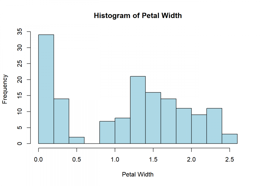
A histogram is a graphical representation of the distribution of a dataset, where data is divided into a set of intervals or bins. The data is represented as vertical bars, with the height of each bar corresponding to the number of data points that fall within a particular bin. Histograms are used to visualize the underlying frequency distribution of a continuous variable, allowing one to identify patterns such as skewness, central tendency, and dispersion.
# Create a histogram of Petal.Width
hist(iris$Petal.Width, main = "Histogram of Petal Width", xlab = "Petal Width", ylab = "Frequency", col = "lightblue", border = "black")
b) Box plot
A box plot, also known as a box-and-whisker plot, is a graphical representation of the distribution and spread of a dataset. It displays five key statistics: the minimum, first quartile (Q1), median (Q2), third quartile (Q3), and maximum. The “box” represents the interquartile range (IQR), which contains the middle 50% of the data, while the “whiskers” extend from the box to the minimum and maximum values. Outliers, if present, are typically represented as individual points outside the whiskers.
# Create a box plot of Petal.Width by Species
boxplot(Petal.Width ~ Species, data = iris, main = "Box plot of Petal Width by Species", xlab = "Species", ylab = "Petal Width")
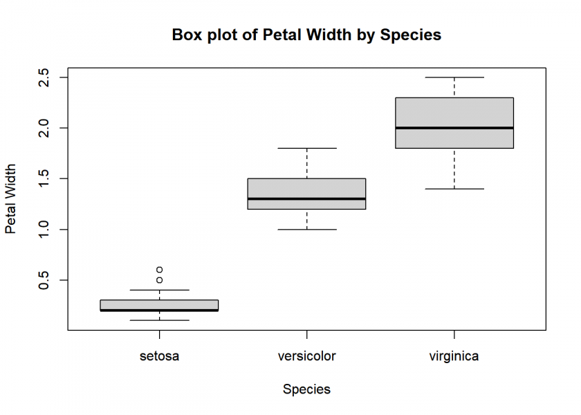
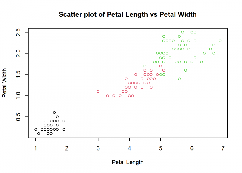
Here, we can very clearly see that petal width indeed separates the different species well. In the following plot, another variable, petal length, is included and the three species are colour-coded.
c) Scatter plot
A scatter plot is a graphical representation of the relationship between two variables, where each data point is represented by a dot on a two-dimensional plane. The horizontal axis (x-axis) represents one variable, while the vertical axis (y-axis) represents the other variable. By analyzing the distribution and pattern of the dots, one can determine the correlation, trends, or outliers between the two variables.
# Create a scatter plot of Petal.Length vs Petal.Width and colour-code Species
plot(iris$Petal.Length, iris$Petal.Width, main = "Scatter plot of Petal Length vs Petal Width", xlab = "Petal Length", ylab = "Petal Width", col = iris$Species)
And, by the way, you can very easily use those plots in other applications (like WinWord or PowerPoint) by clicking on “Export” in Rstudio and then on “Save as Image…” or “Copy to Clipboard…”.
Conclusion
In just 10 minutes, you’ve learned the basics of R using the iris dataset. We covered loading data, data manipulation, and basic plotting. As you continue to explore R, you will discover its vast capabilities and potential for analyzing and visualizing complex data.
To continue on your coding adventure, the following posts are good starting points:
- Learning R: The Ultimate Introduction (incl. Machine Learning!)
- One Rule (OneR) Machine Learning Classification in under One Minute
If you want to dive deeper into data science, I created the following learning path: Learning Path for “Data Science with R” – Part I
Take care, and happy data sleuthing!