Inverse Statistics – and how to create Gain-Loss Asymmetry plots in R

Asset returns have certain statistical properties, also called stylized facts. Important ones are:

• Absence of autocorrelation: basically the direction of the return of one day doesn’t tell you anything useful about the direction of the next day.
• Fat tails: returns are not normal, i.e. there are many more extreme events than there would be if returns were normal.
• Volatility clustering: basically financial markets exhibit high-volatility and low-volatility regimes.
• Leverage effect: high-volatility regimes tend to coincide with falling prices and vice versa.

A good introduction and overview can be found in R. Cont: Empirical properties of asset returns: stylized facts and statistical issues.

One especially fascinating statistical property is the so called gain-loss asymmetry: it basically states that upward movements tend to take a lot longer than downward movements which often come in the form of sudden hefty crashes. So, an abstract illustration of this property would be a sawtooth pattern:

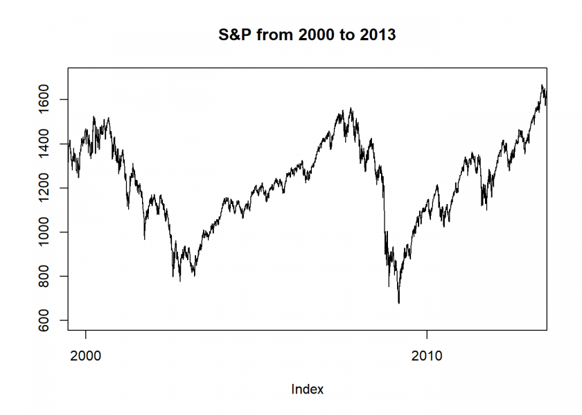
The same effect in real life:

suppressWarnings(suppressMessages(library(quantmod)))
suppressWarnings(suppressMessages(getSymbols("^GSPC", from = "1950-01-01")))
## [1] "GSPC"
plot.zoo(GSPC$GSPC.Close, xlim = c(as.Date("2000-01-01"), as.Date("2013-01-01")), ylim = c(600, 1700), ylab ="", main ="S&P from 2000 to 2013")

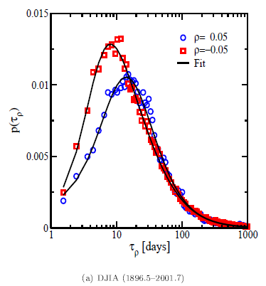
The practical implication for your investment horizon is that your losses often come much faster than your gains (life is just not fair…). To illustrate this authors often plot the investment horizon distribution. It illustrates how long you have to wait for a certain target return, negative as well as positive (for some examples see e.g. here, also the source of the following plot):

This is closely related to what statisticians call first passage time: when is a given threshold passed for the first time? To perform such an analysis you need something called inverse statistics. Normally you would plot the distribution of returns given a fixed time window (= forward statistics). Here we do it the other way around: you fix the return and want to find the shortest waiting time needed to obtain at least the respective return. To achieve that you have to test all possible time windows which can be quite time consuming.

Because I wanted to reproduce those plots I tried to find some code somewhere… to no avail. I then contacted some of the authors of the respective papers… no answer. I finally asked a question on Quantitative Finance StackExchange… and got no satisfying answer either. I therefore wrote the code myself and thereby answered my own question:

inv_stat <- function(symbol, name, target = 0.05) {
  p <- coredata(Cl(symbol))
  end <- length(p)
  days_n <- days_p <- integer(end)
  
  # go through all days and look when target is reached the first time from there
  for (d in 1:end) {
    ret <- cumsum(as.numeric(na.omit(ROC(p[d:end]))))
    cond_n <- ret < -target
    cond_p <- ret > target
    suppressWarnings(days_n[d] <- min(which(cond_n)))
    suppressWarnings(days_p[d] <- min(which(cond_p)))
  }
  
  days_n_norm <- prop.table(as.integer(table(days_n, exclude = "Inf")))
  days_p_norm <- prop.table(as.integer(table(days_p, exclude = "Inf")))
  
  plot(days_n_norm, log = "x", xlim = c(1, 1000), main = paste0(name, " gain-/loss-asymmetry with target ", target), xlab = "days", ylab = "density", col = "red")
  points(days_p_norm, col = "blue")
  
  c(which.max(days_n_norm), which.max(days_p_norm)) # mode of days to obtain (at least) neg. and pos. target return
}

inv_stat(GSPC, name = "S&P 500")

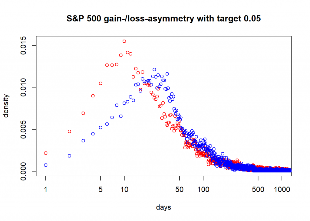
## [1] 10 24

So, here you see that for the S&P 500 since 1950 the mode (peak) of the days to obtain a loss of at least 5% has been 10 days and a gain of the same size 24 days! That is the gain-loss asymmetry in action!

Still two things are missing in the code:

• Detrending of the time series.
• Fitting a probability distribution (the generalized gamma distribution seems to work well).

If you want to add them or if you have ideas how to improve the code, please let me know in the comments! Thank you and stay tuned!