

Here I give a very short introduction on how to use the OneR Machine Learning package for the hurried, so buckle up!
You can also watch this video which goes through the following example step-by-step:
After installing the OneR package from CRAN (install.packages("OneR")) load it
# install.packages("OneR")
library(OneR)
Use the famous Iris dataset and determine optimal bins for numeric data:
data <- optbin(iris)
Build a model with the best predictor:
model <- OneR(data, verbose = TRUE)
##
##     Attribute    Accuracy
## 1 * Petal.Width  96%
## 2   Petal.Length 95.33%
## 3   Sepal.Length 74.67%
## 4   Sepal.Width  55.33%
## ---
## Chosen attribute due to accuracy
## and ties method (if applicable): '*'
Show the learned rules and model diagnostics:
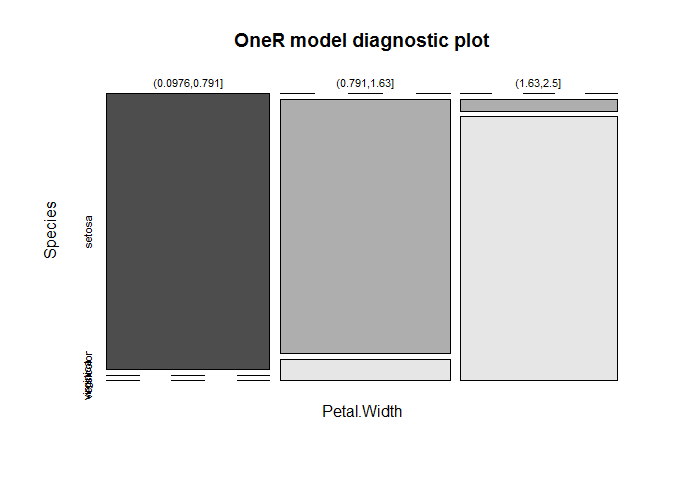
summary(model)
##
## Call:
## OneR(data = data, verbose = TRUE)
##
## Rules:
## If Petal.Width = (0.0976,0.791] then Species = setosa
## If Petal.Width = (0.791,1.63]   then Species = versicolor
## If Petal.Width = (1.63,2.5]     then Species = virginica
##
## Accuracy:
## 144 of 150 instances classified correctly (96%)
##
## Contingency table:
##             Petal.Width
## Species      (0.0976,0.791] (0.791,1.63] (1.63,2.5] Sum
##   setosa               * 50            0          0  50
##   versicolor              0         * 48          2  50
##   virginica               0            4       * 46  50
##   Sum                    50           52         48 150
## ---
## Maximum in each column: '*'
##
## Pearson's Chi-squared test:
## X-squared = 266.35, df = 4, p-value < 2.2e-16
Plot model diagnostics:
plot(model)
Use the model to predict data:
prediction <- predict(model, data)
Evaluate the prediction statistics:
eval_model(prediction, data)
##
## Confusion matrix (absolute):
##             Actual
## Prediction   setosa versicolor virginica Sum
##   setosa         50          0         0  50
##   versicolor      0         48         4  52
##   virginica       0          2        46  48
##   Sum            50         50        50 150
##
## Confusion matrix (relative):
##             Actual
## Prediction   setosa versicolor virginica  Sum
##   setosa       0.33       0.00      0.00 0.33
##   versicolor   0.00       0.32      0.03 0.35
##   virginica    0.00       0.01      0.31 0.32
##   Sum          0.33       0.33      0.33 1.00
##
## Accuracy:
## 0.96 (144/150)
##
## Error rate:
## 0.04 (6/150)
##
## Error rate reduction (vs. base rate):
## 0.94 (p-value < 2.2e-16)
Please note that a very good accuracy of 96% is reached effortlessly.
“Petal.Width” is identified as the attribute with the highest predictive value. The cut points of the intervals are found automatically (via the included optbin function). The results are three very simple, yet accurate, rules to predict the respective species.
The nearly perfect separation of the areas in the diagnostic plot gives a good indication of the model’s ability to separate the different species.
The whole code of this post:
# install.packages("OneR")
library(OneR)
data <- optbin(iris)
model <- OneR(data, verbose = TRUE)
summary(model)
plot(model)
prediction <- predict(model, data)
eval_model(prediction, data)
More sophisticated examples will follow in upcoming posts… so stay tuned!
UPDATE March 19, 2020
For more examples see e.g. our OneR category:
Learning Machines: Category: OneR
I would love to hear about your experiences with the OneR package. Please drop a line or two in the comments – Thank you!
UPDATE September 29, 2021
I created a video for this post (in German):
Some genuinely interesting information, well written and broadly speaking user pleasant.
Thank you very much for your feedback, it is highly appreciated!
Dear Prof Jouanne-Diedrich,
Thanks for the wonderful content you share on this blog and for writing the OneR package.
One question I have about the OneR package:
It would seem that in the case of binary response it’s equivalent to running
rpartwithmaxdedpth = 1?Thank you for your kind words, it is highly appreciated!
Concerning
rpart: this would make sense sinceOneRbasically produces decision trees with depth one. I guess that you would still often get different results due to different discretization schemes (see theoptbinfunction and its different options) and the different handling ofNAvalues.Did you do some tests?
Thank you so much! I appreciate your effort.
So proud
Thank you Alexandra, your feedback is highly appreciated!
Dear Prof Jouanne-Diedrich,
Thanks for creating the OneR pkg.!
Simple and clear always wins…
A suggestion (if I may):
with the vertical bars,
works fine.
But… the Y axis labels:
“versicolor” and “virginica”
overlap each other,
so these words are difficult to read/separate.
Suggested solution:
—————
make the
plot()outputto be =horizontal= bars.
This way,
all 3 Species (categorical) labels
will be easy to read on the plot!…
Thanks / Danke!
Ray
San Francisco
Thank you, Ray, for your kind words. Suggestions are always highly appreciated!
The
plot()function used under the hood of OneR is themosaicplot()function. I designed the output in correspondence to the contingency table. How would you change that to horizontal bars without changing the whole orientation of the plot?A perhaps simpler possibility is to change the orientation of the axis labels. It was a deliberate design decision to not include this as an argument of the
plot()function because this is available in R as a general option (argumentlasin thepar()function) and can be changed like so:The options for
lasare the following:0: always parallel to the axis [default],
1: always horizontal,
2: always perpendicular to the axis,
3: always vertical.
Greetings to San Francisco!
Thanks for the quick reply
and solution.
Yes!, in my opinion,
offers the best visibility
of the 3 Y-axis labels:
(setosa, versicolor, virginica).
And the labels are easy to read
without overlapping !.
Again thank you
for a wonderful easy and useful pkg.
Best wishes and stay safe!.
Ray
San Francisco.
Your video tutural is very helpful. Thank you. I like it.
Questions to OneR:
Error rate reduction=0.94, what’s that? How can I use it?p-value < 2.2e-16, what does p-value mean?tutural–>tutorial
Thank you for your great feedback, highly appreciated.
You can find a thorough answer in “Details” of the
eval_model()function in the documentation of the OneR package.