Learning Data Science: Why a High R^2 Can Be Misleading

A high $R^2$ can make a regression model look impressively accurate — but this number can be deceptive. If you want to understand why a high $R^2$ is not always a sign of a good model, read on!

In the post, Learning Data Science: Modelling Basics, we built a simple model to predict income from age. R printed a model summary containing something called R-squared, but we did not yet discuss what that value actually means.

At first sight, a high $R^2$ looks highly reassuring. In our example, the linear model achieved an $R^2$ close to 90%. That sounds impressive.

However, just as high classification accuracy can be misleading — as discussed in ZeroR: The Simplest Possible Classifier, or Why High Accuracy can be Misleading — a high $R^2$ can also create a false sense of confidence.

To understand why, it helps to examine the formula itself and then revisit the three models from the previous post: the mean model, the linear model, and the polynomial model.

The Meaning of $R^2$

The coefficient of determination is defined as:

$R^2 = 1 - \frac{\sum (y_i-\hat y_i)^2}{\sum (y_i-\bar y)^2}$

At first glance, the formula appears intimidating, but its basic idea is relatively simple.

The denominator

$SS_{tot} = \sum (y_i-\bar y)^2$

measures the total variation in the target variable. It quantifies how strongly the observed values differ from their mean.

The numerator

$SS_{res} = \sum (y_i-\hat y_i)^2$

measures the remaining unexplained error after fitting the model.

Thus, $R^2$ measures the proportion of variation explained by the model.

An $R^2$ of:

0 means the model explains none of the variation,
1 means the model explains all variation perfectly.

This sounds straightforward enough. The difficulty is that perfectly explaining the observed data is not necessarily the same thing as building a useful predictive model.

The Mean Model

Let us begin with the simplest possible regression model.

Suppose we completely ignore age and simply predict the average income for every individual:

$\hat y_i = \bar y$

This is effectively the regression equivalent of ZeroR. The model does not learn any relationship at all.

In this case:

$y_i - \hat y_i = y_i - \bar y$

Therefore, the residual sum of squares becomes identical to the total sum of squares:

$\sum (y_i-\hat y_i)^2 = \sum (y_i-\bar y)^2$

Substituting this into the formula gives:

$R^2 = 1 - \frac{SS_{tot}}{SS_{tot}} = 0$

The model explains none of the variation in the data.

This corresponds to the underfitting case discussed previously: the model is too simple to capture the underlying structure.

The Polynomial Model

Now consider the opposite extreme.

Instead of fitting a straight line, suppose we fit a polynomial of sufficiently high degree. In fact, if we have $n$ observations with distinct age values, a polynomial of degree up to $n-1$ can pass exactly through all observed data points:

$y = a_0 + a_1x + a_2x^2 + \dots + a_{n-1}x^{n-1}$

In that case:

$y_i = \hat y_i$

for all observations, implying:

$\sum (y_i-\hat y_i)^2 = 0$

and therefore:

$R^2 = 1$

The model achieves a perfect fit.

At first sight, this appears ideal. In practice, however, such a model often performs poorly on unseen data because it has adapted itself not only to the underlying relationship, but also to random fluctuations and noise within the training data.

This is the classical overfitting problem.

A perfect $R^2$ may therefore indicate not a particularly good model, but a model that has become too flexible.

The Linear Model

The linear model from the previous post lies between these two extremes.

It is simple enough to avoid memorizing every random fluctuation, yet flexible enough to capture a meaningful trend in the data.

This balance between simplicity and flexibility is one of the central themes in statistical learning.

The idea was summarized in the previous post with the following plot:

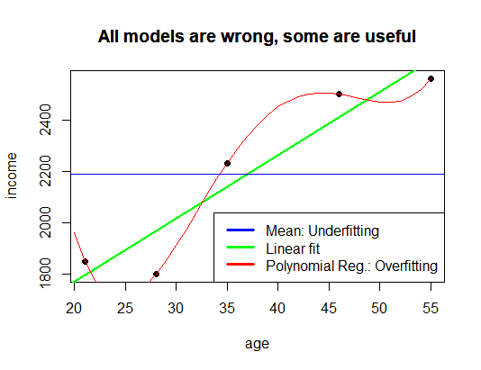
and by the famous observation attributed to George Box:

“All models are wrong, but some are useful.”

The objective in modelling is therefore not to maximize complexity or maximize $R^2$ , but to find a model that generalizes well beyond the observed sample.

Why $R^2$ Alone Is Insufficient

The key limitation of $R^2$ is that it evaluates fit on the observed data only.

It does not directly measure:

predictive performance on unseen data,
robustness,
causal validity, or
generalization ability.

As model complexity increases, $R^2$ almost always increases as well. A sufficiently flexible model can often achieve values very close to 1 even when its predictions on new data are poor.

For this reason, practical data science relies on additional evaluation methods such as:

train-test splits,
cross-validation,
regularization,
adjusted $R^2$ , and
out-of-sample testing.

The goal is not to reproduce historical observations perfectly, but to construct models that remain useful when confronted with new data.

A high $R^2$ can therefore mean two very different things:

the model has identified a genuine structure,
or the model has merely adapted itself too closely to the training data.

Distinguishing between these possibilities is one of the central challenges of machine learning and statistical modelling.

2 thoughts on “Learning Data Science: Why a High R^2 Can Be Misleading”

Pingback: Learning Data Science: Modelling Basics – Learning Machines
Pingback: ZeroR: The Simplest Possible Classifier, or Why High Accuracy can be Misleading – Learning Machines