Learning Data Science: Modelling Basics

Data Science is all about building good models, so let us start by building a very simple model: we want to predict monthly income from age (in a later post we will see that age is indeed a good predictor for income).

For illustrative purposes we just make up some numbers for age and income, load both into a data frame, plot it and calculate its correlation matrix:

age <- c(21, 46, 55, 35, 28)
income <- c(1850, 2500, 2560, 2230, 1800)
data <- data.frame(age, income)
plot(data, pch = 16)

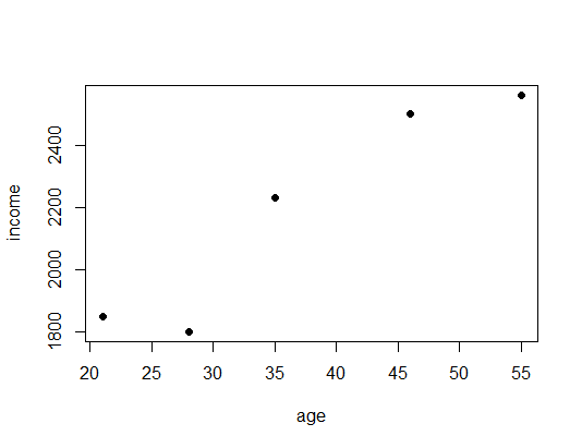
cor(data) # correlation
##              age    income
## age    1.0000000 0.9464183
## income 0.9464183 1.0000000

Just by looking at the plot, we can see that the points seem to be linearly dependent. The correlation matrix corroborates this with a correlation of nearly $95\%$ (for more on correlation see: Causation doesn’t imply Correlation either). To build a linear regression model we use the lm function (for linear model). To specify the model we use the standard R formula interface: on the left-hand side comes the dependent variable, i.e. the variable that we want to predict (income) and on the right-hand side comes the independent variable, i.e. the variable that we want to use to predict income, viz. age – in between both variables we put a tilde (~). After that we plot the model as a line and look at some model diagnostics:

# building linear regression model
LinReg <- lm(income ~ age) # assign model to variable
abline(LinReg, col = "green", lwd = 2) # add regression line

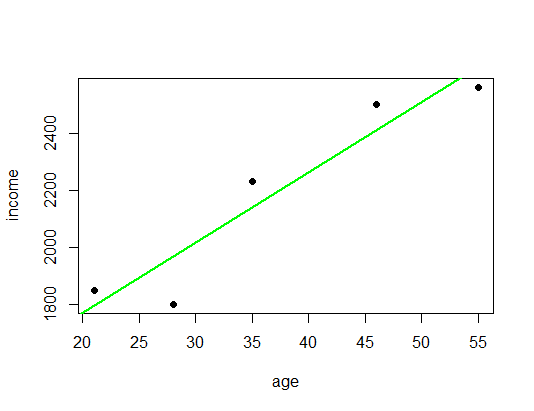
LinReg # coefficients
## 
## Call:
## lm(formula = income ~ age)
## 
## Coefficients:
## (Intercept)          age  
##     1279.37        24.56

summary(LinReg) # model summary
## 
## Call:
## lm(formula = income ~ age)
## 
## Residuals:
##       1       2       3       4       5 
##   54.92   90.98  -70.04   91.12 -166.98 
## 
## Coefficients:
##             Estimate Std. Error t value Pr(>|t|)   
## (Intercept) 1279.367    188.510   6.787  0.00654 **
## age           24.558      4.838   5.076  0.01477 * 
## ---
## Signif. codes:  0 '***' 0.001 '**' 0.01 '*' 0.05 '.' 0.1 ' ' 1
## 
## Residual standard error: 132.1 on 3 degrees of freedom
## Multiple R-squared:  0.8957, Adjusted R-squared:  0.8609 
## F-statistic: 25.77 on 1 and 3 DF,  p-value: 0.01477

The general line equation is $y=mx+b$ , where $m$ is the slope (in this case $24.558$ ) and $b$ the intercept (here $1279.367$ ). The p-values in the last column show us that both parameters are significant, so with a high probability not due to randomness (more on statistical significance can be found here: From Coin Tosses to p-Hacking: Make Statistics Significant Again!). If we now want to predict the income of a 40-year old we just have to calculate $1279.37+40\cdot24.56=2261.67$ .

To do the same calculation in R we can conveniently use the predict function which does this calculation for us automatically. We can also use vectors as input and get several predictions at once. Important is that we use the independent variable with its name as a data frame, otherwise R will throw an error.

# predicting income with linear model
predict(LinReg, data.frame(age = 40))
##       1 
## 2261.67

pred_LinReg <- predict(LinReg, data.frame(age = seq(from = 0, to = 80, by = 5)))
names(pred_LinReg) <- seq(0, 80, 5)
pred_LinReg
##        0        5       10       15       20       25       30       35 
## 1279.367 1402.155 1524.944 1647.732 1770.520 1893.308 2016.097 2138.885 
##       40       45       50       55       60       65       70       75 
## 2261.673 2384.461 2507.249 2630.038 2752.826 2875.614 2998.402 3121.190 
##       80 
## 3243.979

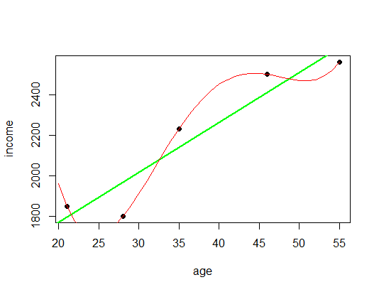
So far so good, but wouldn’t it be nice to actually have a model that is even more accurate, a model where the line actually goes through all the data points so that all the available information is being used. Let us do that with a so-called polynomial regression (in red):

# polynomial regression
PolyReg <- lm(income ~ poly(age, 4, raw = TRUE))
lines(c(20:55), predict(PolyReg, data.frame(age = c(20:55))), col = "red")

pred_PolyReg <- predict(PolyReg, data.frame(age = seq(0, 80, 5)))
names(pred_PolyReg) <- seq(0, 80, 5)
pred_PolyReg
##         0         5        10        15        20        25        30 
## 19527.182 11103.509  5954.530  3164.488  1959.098  1705.541  1912.468 
##        35        40        45        50        55        60        65 
##  2230.000  2449.726  2504.705  2469.464  2560.000  3133.778  4689.732 
##        70        75        80 
##  7868.267 13451.255 22362.037

What do you think? Is this a better model? Well, there is no good reason why income should go up the younger or older you are, and there is no good reason why there should be a bump between $50$ and $55$ . In other words, this model takes the noise as legitimate input which actually makes it worse! To have a good model you always need some rigidity to generalize the data.

This illustration is a good example of one of the big problems of machine learning: overfitting the data! The other extreme would be underfitting, which is included in the following plot as a blue line:

# mean income as a model
abline(h = mean(income), col = "blue")

title(main = "All models are wrong, some are useful")
legend("bottomright", c("Mean: Underfitting", "Linear fit", "Polynomial Reg.: Overfitting"), col = c("blue", "green", "red"), lwd = 3)

mean(income)
## [1] 2188

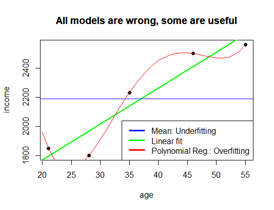
We just took the mean value of income and claimed that no matter the age everybody would earn about $2200$ . This also obviously doesn’t make the cut. In practice and in all data science projects you always have to look for a model that hits the sweet spot between over- and underfitting. This is as much an art as a science, although there are certain best practices like dividing the data into a training and a test set, cross-validation, etc.

Another important point is that all models have their area of applicability. In physics, for example, quantum physics works well for the very small but not very good for the very big, it is the other way round for relativity theory. In this case, we didn’t have data for people of very young or very old age, so it is in general very dangerous to make a prediction for those people, i.e. for values outside of the original observation range (also called extrapolation – in contrast to interpolation, i.e. predictions within the original range). In the case of the linear model, we got an income of about $1280$ for newborns (the intercept)! And the income gets higher the older people get, also something that doesn’t make sense. This behaviour was a lot worse for the non-linear model.

So, here you can see that it is one thing to just let R run and spit something out and quite another one to find a good model and interpret it correctly – even for such a simple problem as this one. In a later post we will use real-world data to predict income brackets with OneR, decision trees, and random forests, so stay tuned!

UPDATE March 19, 2019
The post on now online:
Learning Data Science: Predicting Income Brackets!

UPDATE September 28, 2021
I created a video for this post (in German):