

Forecasting the future has always been one of man’s biggest desires and many approaches have been tried over the centuries. In this post we will look at a simple statistical method for time series analysis, called AR for Autoregressive Model. We will use this method to predict future sales data and will rebuild it to get a deeper understanding of how this method works, so read on!
Let us dive directly into the matter and build an AR model out of the box. We will use the inbuilt BJsales dataset which contains 150 observations of sales data (for more information consult the R documentation). Conveniently enough AR models can be built directly in base R with the ar.ols() function (OLS stands for Ordinary Least Squares which is the method used to fit the actual model). Have a look at the following code:
data <- BJsales
head(data)
## [1] 200.1 199.5 199.4 198.9 199.0 200.2

N <- 3 # how many periods lookback
n_ahead <- 10 # how many periods forecast

# build autoregressive model with ar.ols()
model_ar <- ar.ols(data, order.max = N) # ar-model
pred_ar <- predict(model_ar, n.ahead = n_ahead)
pred_ar$pred
## Time Series:
## Start = 151
## End = 160
## Frequency = 1
##  [1] 263.0299 263.3366 263.6017 263.8507 264.0863 264.3145 264.5372
##  [8] 264.7563 264.9727 265.1868

plot(data, xlim = c(1, length(data) + 15), ylim = c(min(data), max(data) + 10))
lines(pred_ar$pred, col = "blue", lwd = 5)
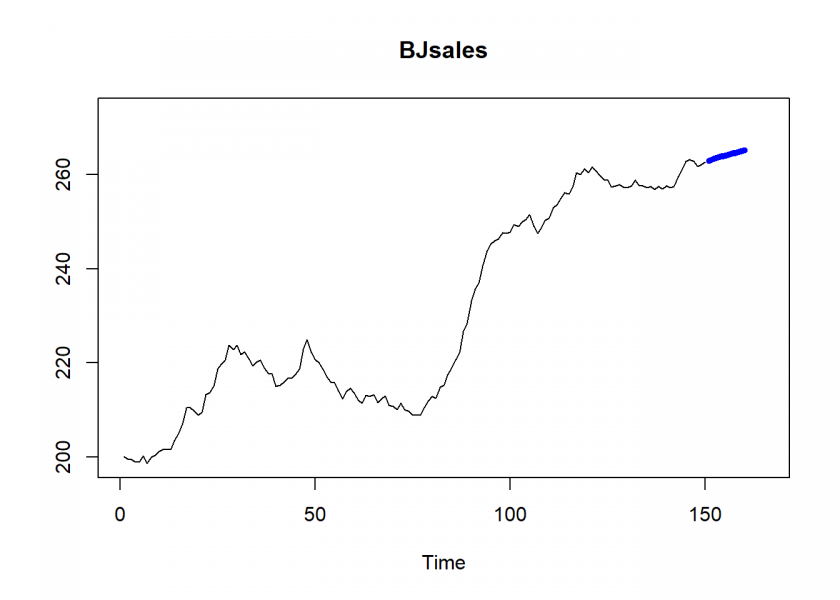
Well, this seems to be good news for the sales team: rising sales! Yet, how does this model arrive at those numbers? To understand what is going on we will now rebuild the model. Basically, everything is in the name already: auto-regressive, i.e. a (linear) regression on (a delayed copy of) itself (auto from Ancient Greek self)!
So, what we are going to do is create a delayed copy of the time series and run a linear regression on it. We will use the lm() function from base R for that (see also Learning Data Science: Modelling Basics). Have a look at the following code:
# reproduce with lm()
df_data <- data.frame(embed(data, N+1) - mean(data))
head(df_data)
##        X1      X2      X3      X4
## 1 -31.078 -30.578 -30.478 -29.878
## 2 -30.978 -31.078 -30.578 -30.478
## 3 -29.778 -30.978 -31.078 -30.578
## 4 -31.378 -29.778 -30.978 -31.078
## 5 -29.978 -31.378 -29.778 -30.978
## 6 -29.678 -29.978 -31.378 -29.778

model_lm <- lm(X1 ~., data = df_data) # lm-model
coeffs <- cbind(c(model_ar$x.intercept, model_ar$ar), coef(model_lm))
coeffs <- cbind(coeffs, coeffs[ , 1] - coeffs[ , 2])
round(coeffs, 12)
##                   [,1]       [,2] [,3]
## (Intercept)  0.2390796  0.2390796    0
## X2           1.2460868  1.2460868    0
## X3          -0.0453811 -0.0453811    0
## X4          -0.2042412 -0.2042412    0

data_pred <- df_data[nrow(df_data), 1:N]
colnames(data_pred) <- names(model_lm$coefficients)[-1]
pred_lm <- numeric()
for (i in 1:n_ahead) {
  data_pred <- cbind(predict(model_lm, data_pred), data_pred)
  pred_lm <- cbind(pred_lm, data_pred[ , 1])
  data_pred <- data_pred[ , 1:N]
  colnames(data_pred) <- names(model_lm$coefficients)[-1]
}

preds <- cbind(pred_ar$pred, as.numeric(pred_lm) + mean(data))
preds <- cbind(preds, preds[ , 1] - preds[ , 2])
colnames(preds) <- NULL
round(preds, 9)
## Time Series:
## Start = 151
## End = 160
## Frequency = 1
##         [,1]     [,2] [,3]
## 151 263.0299 263.0299    0
## 152 263.3366 263.3366    0
## 153 263.6017 263.6017    0
## 154 263.8507 263.8507    0
## 155 264.0863 264.0863    0
## 156 264.3145 264.3145    0
## 157 264.5372 264.5372    0
## 158 264.7563 264.7563    0
## 159 264.9727 264.9727    0
## 160 265.1868 265.1868    0
As you can see, the coefficients and predicted values are the same (except for some negligible rounding errors)!
A few things warrant further attention: When building the linear model in line 17 the formula is created dynamically on the fly because the dependent variable is in the last column which number depends on N (the number of lookback periods). To be more precise, it is not just a simple linear regression but a multiple regression because each column (which represent different time delays) goes into the model as a separate (independent) variable. Additionally, the regression is performed on the demeaned data, meaning that you subtract the mean.
So, under the hood what sounds so impressive (“Autoregressive model”.. wow!) is nothing else but good ol’ linear regression. So, for this method to work, there must be some autocorrelation in the data, i.e. some repeating linear pattern.
As you can imagine there are instances where this will not work. For example, in financial time series there is next to no autocorrelation (otherwise it would be too easy, right! – see also my question and answers on Quant.SE here: Why aren’t econometric models used more in Quant Finance?).
In order to use this model to predict n_ahead periods ahead the predict function first uses the last N periods and then uses the new predicted values as input for the next prediction, and so forth n_ahead times. After that, the mean is added again. Obviously, the farther we predict into the future the more uncertain the forecast becomes because the basis of the prediction comprises more and more values that were predicted themselves. The values for both parameters were taken here for demonstration purposes only. A realistic scenario would be to take more lookback periods than predicted periods and you would, of course, take domain knowledge into account, e.g. when you have monthly data take at least twelve periods as your N.
This post only barely scratched the surface of forecasting time series data. Basically, many of the standard approaches of statistics and machine learning can be modified so that they can be used on time series data. Yet, even the most sophisticated method is not able to foresee external shocks (like the current COVID-19 pandemic) and feedback loops when the very forecasts change the actual behaviour of people.
So, all methods have to be taken with a grain of salt because of those systematic challenges. You should always keep that in mind when you get the latest sales forecast!
One thought on “Time Series Analysis: Forecasting Sales Data with Autoregressive (AR) Models”