Kalman Filter as a Form of Bayesian Updating

The Kalman filter is a very powerful algorithm to optimally include uncertain information from a dynamically changing system to come up with the best educated guess about the current state of the system. Applications include (car) navigation and stock forecasting. If you want to understand how a Kalman filter works and build a toy example in R, read on!

The following post is based on the post “Das Kalman-Filter einfach erklärt” which is written in German and uses Matlab code (so basically two languages nobody is interested in any more 😉 ). This post is itself based on an online course “Artificial Intelligence for Robotics” by my colleague Professor Sebastian Thrun of Standford University.

Because we are dealing with uncertainty here, we need a probability distribution. A good choice often is a Gaussian or normal distribution. It is defined by two parameters, the mean and the variance (or standard deviation which is just the square root of the variance). These two parameters have to be updated by incoming information which is itself uncertain.

This can be interpreted as some form of Bayesian updating (if you want to learn more about Bayes and his famous formula, you can read two former posts of mine here: Base Rate Fallacy – or why No One is justified to believe that Jesus rose and Learning Data Science: Sentiment Analysis with Naive Bayes).

Professor Thrun explains (just ignore the quiz at the end of the video):

The update step in R code:

update <- function(mean1, var1, mean2, var2) {
  # calculates new position as multiplication of two Gaussians:
  # prior probability and new information (noisy measurement)
  new_mean <- (var2*mean1 + var1*mean2) / (var1 + var2)
  new_var <- 1/(1/var1 + 1/var2)
  return(c(new_mean, new_var))
}

After calculating the position based on new information we also have to take into account the motion itself, this is done in the prediction step:

Here is the R implementation:

predict <- function(mean1, var1, mean2, var2) {
  # Calculates new postion as sum (= convolution) of two Gaussians:
  # prior probability and new information (noisy movement)
  new_mean <- mean1 + mean2
  new_var  <- var1 + var2
  return(c(new_mean, new_var))
}

Now, we are putting both steps together to form a cycle:

As an example let us create a trajectory along a sine wave with measurements and motion affected by noise (= uncertainty):

var_measure <- 5 # variance measure
var_motion <- 2 # variance motion
pos <- c(0, 10000) # Starting values position and variance

## Kalman calculation
set.seed(123)
pos_real <- 10 * sin(seq(1, 20, 0.1))
motion_real <- diff(pos_real)
measure <- pos_real + rnorm(length(pos_real), 0, sqrt(var_measure))
motion <- motion_real + rnorm(length(motion_real), 0, sqrt(var_motion))
kalman_update <- c()

for (i in 1:length(measure)) {
  pos <- update(pos[1], pos[2], measure[i], var_measure)
  kalman_update <- c(kalman_update, pos[1])
  pos <- predict(pos[1], pos[2], motion[i], var_motion)
}

plot(measure, col = "red")
lines(kalman_update, col = "blue")
lines(pos_real, col = "black")

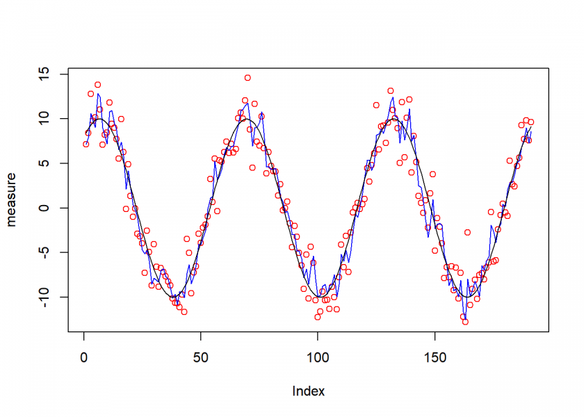
As you can see the resulting blue curve is much more stable than the noisy measurements (small red circles)!

If you want to read about another algorithm (RANSAC) that is able to handle noisy measurements, you can find it here: Separating the Signal from the Noise: Robust Statistics for Pedestrians.

In any case, stay tuned for more to come!