One of the most notoriously difficult subjects in statistics is the concept of statistical tests. We will explain the ideas behind it step by step to give you some intuition on how to use (and misuse) it, so read on…
You can also watch the video for this post (in German):
Let us begin with some coin tosses and the question of how to find out whether a coin is fair, i.e. shows heads and tails with fifty-fifty probability. If you had all the time of the world you could throw it indefinitely often to see where the probabilities stabilize. Yet, in reality we only have some sample of tosses and have to infer results based on this. Because of this the area that deals with those problems is called inferential statistics (also inductive statistics).
So, to keep things simple, let us throw our coin only ten times. Where is the point where you would suspect that something is not quite right with this coin? As soon as you don’t get five times heads and five times tails? Or only when you get ten times one side only? Possibly somewhere in between? But where exactly?
The first thing to understand is that this is a somewhat arbitrary decision… but one that should be set in advance, and which should adhere to some general standard. The idea is to set some fixed probability with which you compare the probability of the result you see in your experiment (i.e. the number of heads and tails in our example). When you obtain a result that is as improbable or even more so than that pre-fixed probability you conclude that the result happened not just by chance but that something significant happened (e.g. that your coin is unfair). The generally accepted probability below which one speaks of a significant result is 5% (or 0.05), it is therefore called significance level.
After fixing the significance level at 0.05 we have to compare it with the probability of our observed result (or a result that is even more extreme). Let us say that we got nine times one side of the coin and only one time the other. What is the probability of getting this or an even more extreme result? The general probability formula is:
![]()
For the numerator, we get 22 possibilities for observing the above-mentioned or an even more extreme result: two times ten possibilities that each of the ten coins could be the odd one out and two more extreme cases showing only heads or only tails. For the denominator we get ![]() possibilities for throwing
possibilities for throwing ![]() coins:
coins:
22 / 2^10
## [1] 0.02148438
So, the probability is about 2% which is below 5%, so we would conclude that our coin is not fair!
Another possibility is to use the binomial coefficient which gives us the number of possibilities to choose k items out of n items (to understand the binomial coefficient see also: Learning R: Permutations and Combinations with Base R). Conveniently enough the R function is called choose(n, k):
(choose(10, 0) + choose(10, 1) + choose(10, 9) + choose(10, 10))/2^10
## [1] 0.02148438
Or, because the situation is symmetric:
2 * (choose(10, 0) + choose(10, 1))/2^10
## [1] 0.02148438
To make things even simpler we can use the binomial distribution for our calculation, where basically all of the needed binomial coefficients are summed up automatically:
prob <- 0.5 # fair coin
n <- 10     # number of coin tosses
k <- 1      # number of "successes", i.e. how many coins show a different side than the rest

2 * pbinom(k, n, prob)
## [1] 0.02148438
As you can see, we get the same probability value over and over again. If you have understood the line of thought so far you are ready for the last step: performing the statistical test with the binom.test() function:
binom.test(k, n)
##
##  Exact binomial test
##
## data:  k and n
## number of successes = 1, number of trials = 10, p-value = 0.02148
## alternative hypothesis: true probability of success is not equal to 0.5
## 95 percent confidence interval:
##  0.002528579 0.445016117
## sample estimates:
## probability of success
##                    0.1
As you can see, we get the same number again: it is named p-value in the output:
The p-value is the probability of getting the observed – or an even more extreme – result under the condition that the null hypothesis is true.
The only thing that is new here is the null hypothesis. The null hypothesis (or H0 hypothesis) is just a fancy name for the assumption that in general things are unremarkable, examples could be: our coin is fair, a new medical drug doesn’t work (its effect is just random noise) or one group of students is not better than the other. In practice, we would often take the opposite of what we would like to examine as our H0. Why? Because if you want to examine something you cannot assume it to be true to begin with. Another more practical reason is that oftentimes you would not be able to calculate the p-value because you don’t know the strength of the effect, i.e. how unfair the coin is.
So, after having a look at the output we would formally say that we have a significant result and therefore reject the null hypothesis that the coin is fair.
In most real-world scenarios the situation is not that clear-cut as it is with our coins. Therefore we won’t normally use a binomial test but the workhorse of statistical inference: the famous t-test! On the positive side, you can use the t-test in many situations where you don’t have all the information on the underlying population distribution, e.g. its variance. It is based on comparatively mild assumptions, e.g. that the population distribution is normal (which is itself effectively based on the Central Limit Theorem, to read more see: The Central Limit Theorem (CLT): From Perfect Symmetry to the Normal Distribution) – and even this can be relaxed as long as its variance is finite and when you have big sample sizes. If it is normal though small sample sizes suffice. On the negative side the t-test often only gives approximations of exact tests. Yet the bigger the sample sizes the better the approximation. Enough of the theory, let us perform a t-test with our data. We use the t.test() function for that:
data <- c(rep(0, n-k), rep(1, k))
t.test(data, mu = prob)
##
##  One Sample t-test
##
## data:  data
## t = -4, df = 9, p-value = 0.00311
## alternative hypothesis: true mean is not equal to 0.5
## 95 percent confidence interval:
##  -0.1262157  0.3262157
## sample estimates:
## mean of x
##       0.1
As you can see, we get a different p-value this time but the test is still significant and leads to the right conclusion. As said before, the bigger the sample size the better the approximation.
Let us try two more examples. First we use the inbuilt mtcars dataset to test whether petrol consumption of manual and automatic transmissions differ significantly:
head(mtcars)
##                    mpg cyl disp  hp drat    wt  qsec vs am gear carb
## Mazda RX4         21.0   6  160 110 3.90 2.620 16.46  0  1    4    4
## Mazda RX4 Wag     21.0   6  160 110 3.90 2.875 17.02  0  1    4    4
## Datsun 710        22.8   4  108  93 3.85 2.320 18.61  1  1    4    1
## Hornet 4 Drive    21.4   6  258 110 3.08 3.215 19.44  1  0    3    1
## Hornet Sportabout 18.7   8  360 175 3.15 3.440 17.02  0  0    3    2
## Valiant           18.1   6  225 105 2.76 3.460 20.22  1  0    3    1

# make new column with better labels
mtcars$trans <- ifelse(mtcars$am == 0, "aut", "man")
mtcars$trans <- factor(mtcars$trans)

mtcars$mpg
##  [1] 21.0 21.0 22.8 21.4 18.7 18.1 14.3 24.4 22.8 19.2 17.8 16.4 17.3 15.2
## [15] 10.4 10.4 14.7 32.4 30.4 33.9 21.5 15.5 15.2 13.3 19.2 27.3 26.0 30.4
## [29] 15.8 19.7 15.0 21.4

mtcars$trans
##  [1] man man man aut aut aut aut aut aut aut aut aut aut aut aut aut aut
## [18] man man man aut aut aut aut aut man man man man man man man
## Levels: aut man

by(mtcars$mpg, mtcars$trans, summary)
## mtcars$trans: aut
##    Min. 1st Qu.  Median    Mean 3rd Qu.    Max.
##   10.40   14.95   17.30   17.15   19.20   24.40
## --------------------------------------------------------
## mtcars$trans: man
##    Min. 1st Qu.  Median    Mean 3rd Qu.    Max.
##   15.00   21.00   22.80   24.39   30.40   33.90

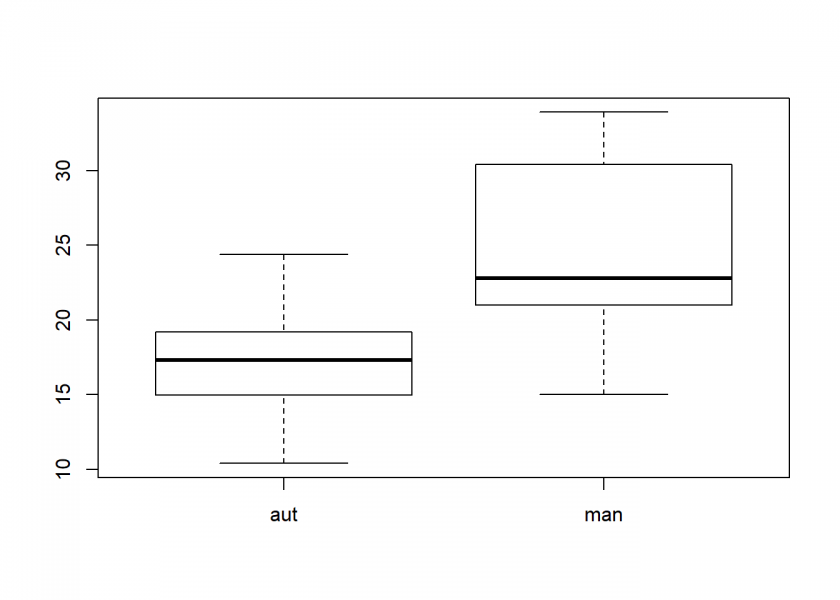
boxplot(mpg ~ trans, data = mtcars)

As we can see the consumption is obviously different – but is it also significantly different at the 5% significance level? Let us find out:
M <- mtcars$trans == "man" #manual
mpg_man <- mtcars[M, ]$mpg #consumption of manual transmission
mpg_man
##  [1] 21.0 21.0 22.8 32.4 30.4 33.9 27.3 26.0 30.4 15.8 19.7 15.0 21.4

mpg_aut <- mtcars[!M, ]$mpg #consumption of automatic transmission
mpg_aut
##  [1] 21.4 18.7 18.1 14.3 24.4 22.8 19.2 17.8 16.4 17.3 15.2 10.4 10.4 14.7
## [15] 21.5 15.5 15.2 13.3 19.2

t.test(mpg_man, mpg_aut)
##
##  Welch Two Sample t-test
##
## data:  mpg_man and mpg_aut
## t = 3.7671, df = 18.332, p-value = 0.001374
## alternative hypothesis: true difference in means is not equal to 0
## 95 percent confidence interval:
##   3.209684 11.280194
## sample estimates:
## mean of x mean of y
##  24.39231  17.14737
Yes, it is significantly different!
And now for our final example, a classic use of the t-test to find out whether a medical drug has a significant effect (we use the inbuilt sleep dataset):
sleep
##    extra group ID
## 1    0.7     1  1
## 2   -1.6     1  2
## 3   -0.2     1  3
## 4   -1.2     1  4
## 5   -0.1     1  5
## 6    3.4     1  6
## 7    3.7     1  7
## 8    0.8     1  8
## 9    0.0     1  9
## 10   2.0     1 10
## 11   1.9     2  1
## 12   0.8     2  2
## 13   1.1     2  3
## 14   0.1     2  4
## 15  -0.1     2  5
## 16   4.4     2  6
## 17   5.5     2  7
## 18   1.6     2  8
## 19   4.6     2  9
## 20   3.4     2 10

by(sleep$extra, sleep$group, summary)
## sleep$group: 1
##    Min. 1st Qu.  Median    Mean 3rd Qu.    Max.
##  -1.600  -0.175   0.350   0.750   1.700   3.700
## --------------------------------------------------------
## sleep$group: 2
##    Min. 1st Qu.  Median    Mean 3rd Qu.    Max.
##  -0.100   0.875   1.750   2.330   4.150   5.500

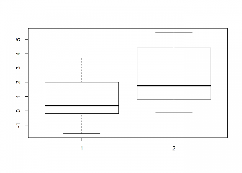
boxplot(extra ~ group, sleep)

Again, there is obviously a difference… but is it significant?
t.test(extra ~ group, sleep)
##
##  Welch Two Sample t-test
##
## data:  extra by group
## t = -1.8608, df = 17.776, p-value = 0.07939
## alternative hypothesis: true difference in means is not equal to 0
## 95 percent confidence interval:
##  -3.3654832  0.2054832
## sample estimates:
## mean in group 1 mean in group 2
##            0.75            2.33
The p-value is above 0.05 which means that this time it cannot be ruled out that the difference is random!
As you can imagine whenever there is money to be made people get creative on how to game the system… unfortunately statistical tests are no exception. Especially in the medical field huge amounts of money are at stake, so one should be well aware of a manipulation technique called p-hacking (also known under the names data snooping or data dredging)!
To summarize our journey into statistical testing so far we have seen that you set a significance level (normally at 0.05) and draw a random sample. You calculate how probable the drawing of this sample (or an even more extreme sample) is and compare it to the significance level. If the probability is below the significance level you say that the test shows a significant result, otherwise you say that one cannot rule out that the difference (if there is one) is just due to chance.
Now, if you don’t like the result… why not draw a sample again? And again? And again? This is p-hacking! Just draw a lot of samples and take the one that fits your agenda!
Of course, this is a stark misuse of the idea of statistical tests. But the fact remains that sometimes samples will be significant just by chance!
In the following example we “prove” that homeopathy works after all (as we all know it just doesn’t work beyond the so-called placebo effect as numerous high-quality studies over many decades have shown). For that end we just conduct one hundred trials and take one out that fits our bill:
p_hack <- function() {
  homeopathy <- rnorm(20, 1.2, 5)
  t.test(homeopathy, mu = 1.2)$p.value
}

set.seed(123)
trials <- replicate(100, p_hack())
trials[6] # homeopathy works!
## [1] 0.033461758

# wait... no it doesn't!
trials
##   [1] 0.522741341 0.785376466 0.624588751 0.587983281 0.057318309
##   [6] 0.033461758 0.876112179 0.461733176 0.495169397 0.519897894
##  [11] 0.800638084 0.836667733 0.915272904 0.340430844 0.087656634
##  [16] 0.879783049 0.824428157 0.784957654 0.898447738 0.494603038
##  [21] 0.279707663 0.438005042 0.886043148 0.158778621 0.167712182
##  [26] 0.135880072 0.185375902 0.662883154 0.840370636 0.331157973
##  [31] 0.283332330 0.423746570 0.849937345 0.503256673 0.546014504
##  [36] 0.725568387 0.727886195 0.167482514 0.586386335 0.493916303
##  [41] 0.937060320 0.271651762 0.236448565 0.191925375 0.983841382
##  [46] 0.373146285 0.520463358 0.323242616 0.193315250 0.757835487
##  [51] 0.429311063 0.284986685 0.868272041 0.844042454 0.885548528
##  [56] 0.996021648 0.978855283 0.588192375 0.495521737 0.610192393
##  [61] 0.242524547 0.404220265 0.136245145 0.004912541 0.408530447
##  [66] 0.458030143 0.784011725 0.357773131 0.818207705 0.698330582
##  [71] 0.451268449 0.740943226 0.266786179 0.120894921 0.050307044
##  [76] 0.387838555 0.232600995 0.834739682 0.669270240 0.516910985
##  [81] 0.273077802 0.291004360 0.369842912 0.132130995 0.454371585
##  [86] 0.567029545 0.219163798 0.524362414 0.737950629 0.855945701
##  [91] 0.959611992 0.901298484 0.931203165 0.204489683 0.843491761
##  [96] 0.567982673 0.329414884 0.107350495 0.911279358 0.696661191
Lo and behold: trial no. 6 shows a significant result – although by design both means are the same (1.2)! So we take this study, publish it and sell lots and lots of useless homeopathy drugs!
How many significant results will we get just by chance on average? Well, exactly the amount of our significance level!
trials <- replicate(1e5, p_hack())
round(length(trials[trials < 0.05]) / length(trials), 2)
## [1] 0.05
As always our friends over at xkcd summarize the situation brilliantly:

UPDATE October 6, 2020
For how to use these ideas to make quick calculations on the back of an envelope see this post:
3.84 or: How to Detect BS (Fast).

Very well written article easily understandable to a layman.
Thank you very much, Rohit – I really appreciate it!
This article opens my eyes to a new world and lets me to know more about statistics.
Thank you, that is very generous of you!
Great article! Couldn’t be more didactic. Thank you.
Thank you, Otavio, highly appreciated!
How comes the number 22 in “we get 22 possibilities for observing the above-mentioned or an even more extreme result”?
There are ten possibilities each for having one coin H (T) and nine coins T (H) = 20
There are two possibilities for having ten coins H (T).
Does this make it clear?