

There are a million reasons to learn R (see e.g. Why R for Data Science – and not Python?), but where to start? I present to you the ultimate introduction to bring you up to speed! So read on…
I call it ultimate because it is the essence of many years of teaching R… or put differently: it is the kind of introduction I would have liked to have when I started out with R back in the days!
A word of warning though: this is an introduction to R and not to statistics, so I won’t explain the statistics terms used here. You do not need to know any other programming language but it does no harm either. Ok, now let us start!
First you need to install R (R Project) and preferably RStudio as a Graphical User Interface (GUI): RStudio Desktop. Both are free and available for all common operating systems.
To get a quick overview of RStudio watch this video:
You can either type in the following commands in the console or open a new script tab (File -> New File -> R Script) and run the commands by pressing Ctrl + Enter/Return after having typed them.
First of all R is a very good calculator:
2 + 2
## [1] 4

sin(0.5)
## [1] 0.4794255

abs(-10) # absolute value
## [1] 10

pi
## [1] 3.141593

exp(1) # e
## [1] 2.718282

factorial(6)
## [1] 720
By the way: The hash is used for comments, everything after it will be ignored!
Of course you can define variables and use them in your calculations:
n1 <- 2
n2 <- 3
n1 # show content of variable by just typing the name
## [1] 2

n1 + n2
## [1] 5

n1 * n2
## [1] 6

n1^n2
## [1] 8
Part of R’s power stems from the fact that functions can handle several numbers at once, called vectors, and do calculations on them. In fact even single numbers are vectors with one element internally. When calling a function arguments are passed with round brackets:
n3 <- c(12, 5, 27) # concatenate (combine) elements into a vector
n3
## [1] 12  5 27

min(n3)
## [1] 5

max(n3)
## [1] 27

sum(n3)
## [1] 44

mean(n3)
## [1] 14.66667

sd(n3) # standard deviation
## [1] 11.23981

var(n3) # variance
## [1] 126.3333

median(n3)
## [1] 12

n3 / c(1, 2, 3) # elementwise operation
## [1] 12.0  2.5  9.0

n3 / 12 # element 12 is recycled
## [1] 1.0000000 0.4166667 2.2500000
In the last example the 12 was recycled three times. R always tries to do that (when feasible), sometimes giving a warning when it might not be intended:
n3 / c(3, 2)
## Warning in n3 / c(3, 2): longer object length is not a multiple of shorter
## object length
## [1] 4.0 2.5 9.0
In cases you only want parts of your vectors you can apply subsetting with square brackets:
n3[1]
## [1] 12

n3[c(2, 3)]
## [1]  5 27
Ranges can easily be created with a colon (for more complex ranges you can use the seq function):
n4 <- 10:20
n4
##  [1] 10 11 12 13 14 15 16 17 18 19 20
When you test whether this vector is bigger than a certain number (i.e. a so-called conditional in computer lingo) you will get logicals (i.e. TRUE or FALSE) as a result. You can use those logicals for subsetting:
n4 > 15
##  [1] FALSE FALSE FALSE FALSE FALSE FALSE  TRUE  TRUE  TRUE  TRUE  TRUE

n4[n4 > 15]
## [1] 16 17 18 19 20
Perhaps you have heard the story of little Gauss where his teacher gave him the task to add all numbers from 1 to 100 to keep him busy for a while? Well, he found a mathematical trick to add them within seconds… for us normal people we can use R:
sum(1:100)
## [1] 5050
When we want to use some code several times we can define our own function (a user-defined function). We do that the same way we create a vector (or any other data structure) because R is a so called functional programming language and functions are so called first-class citizens (i.e. on the same level as other data structures like vectors – if you want to learn more see: Learning R: A Gentle Introduction to Higher-Order Functions). The code that is being executed is put in curly brackets:
gauss <- function(x) {
  sum(1:x)
}
gauss(100)
## [1] 5050

gauss(1000)
## [1] 500500
Of course we also have other data types, e.g. matrices are basically two dimensional vectors:
M <- matrix(1:12, nrow = 3, byrow = TRUE) # create a matrix
M
##      [,1] [,2] [,3] [,4]
## [1,]    1    2    3    4
## [2,]    5    6    7    8
## [3,]    9   10   11   12

dim(M)
## [1] 3 4
Subsetting now has to provide two numbers, the first for the row, the second for the column: [rows, columns], like in the game Battleship. If you leave one of those numbers out, the respective dimension isn’t filtered:
M[2, 3]
## [1] 7

M[ , c(1, 3)]
##      [,1] [,2]
## [1,]    1    3
## [2,]    5    7
## [3,]    9   11
Another possibility to create matrices out of existing vectors:
v1 <- 1:4
v2 <- 4:1
M1 <- rbind(v1, v2) # row bind
M1
##    [,1] [,2] [,3] [,4]
## v1    1    2    3    4
## v2    4    3    2    1

M2 <- cbind(v1, v2)  # column bind
M2
##      v1 v2
## [1,]  1  4
## [2,]  2  3
## [3,]  3  2
## [4,]  4  1
Naming rows, here with inbuilt datasets:
rownames(M2) <- LETTERS[1:4]
M2
##   v1 v2
## A  1  4
## B  2  3
## C  3  2
## D  4  1

LETTERS
##  [1] "A" "B" "C" "D" "E" "F" "G" "H" "I" "J" "K" "L" "M" "N" "O" "P" "Q"
## [18] "R" "S" "T" "U" "V" "W" "X" "Y" "Z"

letters
##  [1] "a" "b" "c" "d" "e" "f" "g" "h" "i" "j" "k" "l" "m" "n" "o" "p" "q"
## [18] "r" "s" "t" "u" "v" "w" "x" "y" "z"
When some result is Not Available (which is also used for missing values):
LETTERS[50]
## [1] NA
Getting the structure of your variables:
str(LETTERS)
##  chr [1:26] "A" "B" "C" "D" "E" "F" "G" "H" "I" "J" "K" "L" "M" "N" ...

str(M2)
##  int [1:4, 1:2] 1 2 3 4 4 3 2 1
##  - attr(*, "dimnames")=List of 2
##   ..$ : chr [1:4] "A" "B" "C" "D"
##   ..$ : chr [1:2] "v1" "v2"
Another famous dataset that is also built into base R is the (iris) dataset, something like an “Hello World!”-equivalent in the data science world (as an aside: if you want to know more about any function or dataset just put the cursor in it and press F1):
iris ## Sepal.Length Sepal.Width Petal.Length Petal.Width Species ## 1 5.1 3.5 1.4 0.2 setosa ## 2 4.9 3.0 1.4 0.2 setosa ## 3 4.7 3.2 1.3 0.2 setosa ## 4 4.6 3.1 1.5 0.2 setosa ## 5 5.0 3.6 1.4 0.2 setosa ## 6 5.4 3.9 1.7 0.4 setosa ## 7 4.6 3.4 1.4 0.3 setosa ## 8 5.0 3.4 1.5 0.2 setosa ## 9 4.4 2.9 1.4 0.2 setosa ## 10 4.9 3.1 1.5 0.1 setosa ## 11 5.4 3.7 1.5 0.2 setosa ## 12 4.8 3.4 1.6 0.2 setosa ## 13 4.8 3.0 1.4 0.1 setosa ## 14 4.3 3.0 1.1 0.1 setosa ## 15 5.8 4.0 1.2 0.2 setosa ## 16 5.7 4.4 1.5 0.4 setosa ## 17 5.4 3.9 1.3 0.4 setosa ## 18 5.1 3.5 1.4 0.3 setosa ## 19 5.7 3.8 1.7 0.3 setosa ## 20 5.1 3.8 1.5 0.3 setosa ## 21 5.4 3.4 1.7 0.2 setosa ## 22 5.1 3.7 1.5 0.4 setosa ## 23 4.6 3.6 1.0 0.2 setosa ## 24 5.1 3.3 1.7 0.5 setosa ## 25 4.8 3.4 1.9 0.2 setosa ## 26 5.0 3.0 1.6 0.2 setosa ## 27 5.0 3.4 1.6 0.4 setosa ## 28 5.2 3.5 1.5 0.2 setosa ## 29 5.2 3.4 1.4 0.2 setosa ## 30 4.7 3.2 1.6 0.2 setosa ## 31 4.8 3.1 1.6 0.2 setosa ## 32 5.4 3.4 1.5 0.4 setosa ## 33 5.2 4.1 1.5 0.1 setosa ## 34 5.5 4.2 1.4 0.2 setosa ## 35 4.9 3.1 1.5 0.2 setosa ## 36 5.0 3.2 1.2 0.2 setosa ## 37 5.5 3.5 1.3 0.2 setosa ## 38 4.9 3.6 1.4 0.1 setosa ## 39 4.4 3.0 1.3 0.2 setosa ## 40 5.1 3.4 1.5 0.2 setosa ## 41 5.0 3.5 1.3 0.3 setosa ## 42 4.5 2.3 1.3 0.3 setosa ## 43 4.4 3.2 1.3 0.2 setosa ## 44 5.0 3.5 1.6 0.6 setosa ## 45 5.1 3.8 1.9 0.4 setosa ## 46 4.8 3.0 1.4 0.3 setosa ## 47 5.1 3.8 1.6 0.2 setosa ## 48 4.6 3.2 1.4 0.2 setosa ## 49 5.3 3.7 1.5 0.2 setosa ## 50 5.0 3.3 1.4 0.2 setosa ## 51 7.0 3.2 4.7 1.4 versicolor ## 52 6.4 3.2 4.5 1.5 versicolor ## 53 6.9 3.1 4.9 1.5 versicolor ## 54 5.5 2.3 4.0 1.3 versicolor ## 55 6.5 2.8 4.6 1.5 versicolor ## 56 5.7 2.8 4.5 1.3 versicolor ## 57 6.3 3.3 4.7 1.6 versicolor ## 58 4.9 2.4 3.3 1.0 versicolor ## 59 6.6 2.9 4.6 1.3 versicolor ## 60 5.2 2.7 3.9 1.4 versicolor ## 61 5.0 2.0 3.5 1.0 versicolor ## 62 5.9 3.0 4.2 1.5 versicolor ## 63 6.0 2.2 4.0 1.0 versicolor ## 64 6.1 2.9 4.7 1.4 versicolor ## 65 5.6 2.9 3.6 1.3 versicolor ## 66 6.7 3.1 4.4 1.4 versicolor ## 67 5.6 3.0 4.5 1.5 versicolor ## 68 5.8 2.7 4.1 1.0 versicolor ## 69 6.2 2.2 4.5 1.5 versicolor ## 70 5.6 2.5 3.9 1.1 versicolor ## 71 5.9 3.2 4.8 1.8 versicolor ## 72 6.1 2.8 4.0 1.3 versicolor ## 73 6.3 2.5 4.9 1.5 versicolor ## 74 6.1 2.8 4.7 1.2 versicolor ## 75 6.4 2.9 4.3 1.3 versicolor ## 76 6.6 3.0 4.4 1.4 versicolor ## 77 6.8 2.8 4.8 1.4 versicolor ## 78 6.7 3.0 5.0 1.7 versicolor ## 79 6.0 2.9 4.5 1.5 versicolor ## 80 5.7 2.6 3.5 1.0 versicolor ## 81 5.5 2.4 3.8 1.1 versicolor ## 82 5.5 2.4 3.7 1.0 versicolor ## 83 5.8 2.7 3.9 1.2 versicolor ## 84 6.0 2.7 5.1 1.6 versicolor ## 85 5.4 3.0 4.5 1.5 versicolor ## 86 6.0 3.4 4.5 1.6 versicolor ## 87 6.7 3.1 4.7 1.5 versicolor ## 88 6.3 2.3 4.4 1.3 versicolor ## 89 5.6 3.0 4.1 1.3 versicolor ## 90 5.5 2.5 4.0 1.3 versicolor ## 91 5.5 2.6 4.4 1.2 versicolor ## 92 6.1 3.0 4.6 1.4 versicolor ## 93 5.8 2.6 4.0 1.2 versicolor ## 94 5.0 2.3 3.3 1.0 versicolor ## 95 5.6 2.7 4.2 1.3 versicolor ## 96 5.7 3.0 4.2 1.2 versicolor ## 97 5.7 2.9 4.2 1.3 versicolor ## 98 6.2 2.9 4.3 1.3 versicolor ## 99 5.1 2.5 3.0 1.1 versicolor ## 100 5.7 2.8 4.1 1.3 versicolor ## 101 6.3 3.3 6.0 2.5 virginica ## 102 5.8 2.7 5.1 1.9 virginica ## 103 7.1 3.0 5.9 2.1 virginica ## 104 6.3 2.9 5.6 1.8 virginica ## 105 6.5 3.0 5.8 2.2 virginica ## 106 7.6 3.0 6.6 2.1 virginica ## 107 4.9 2.5 4.5 1.7 virginica ## 108 7.3 2.9 6.3 1.8 virginica ## 109 6.7 2.5 5.8 1.8 virginica ## 110 7.2 3.6 6.1 2.5 virginica ## 111 6.5 3.2 5.1 2.0 virginica ## 112 6.4 2.7 5.3 1.9 virginica ## 113 6.8 3.0 5.5 2.1 virginica ## 114 5.7 2.5 5.0 2.0 virginica ## 115 5.8 2.8 5.1 2.4 virginica ## 116 6.4 3.2 5.3 2.3 virginica ## 117 6.5 3.0 5.5 1.8 virginica ## 118 7.7 3.8 6.7 2.2 virginica ## 119 7.7 2.6 6.9 2.3 virginica ## 120 6.0 2.2 5.0 1.5 virginica ## 121 6.9 3.2 5.7 2.3 virginica ## 122 5.6 2.8 4.9 2.0 virginica ## 123 7.7 2.8 6.7 2.0 virginica ## 124 6.3 2.7 4.9 1.8 virginica ## 125 6.7 3.3 5.7 2.1 virginica ## 126 7.2 3.2 6.0 1.8 virginica ## 127 6.2 2.8 4.8 1.8 virginica ## 128 6.1 3.0 4.9 1.8 virginica ## 129 6.4 2.8 5.6 2.1 virginica ## 130 7.2 3.0 5.8 1.6 virginica ## 131 7.4 2.8 6.1 1.9 virginica ## 132 7.9 3.8 6.4 2.0 virginica ## 133 6.4 2.8 5.6 2.2 virginica ## 134 6.3 2.8 5.1 1.5 virginica ## 135 6.1 2.6 5.6 1.4 virginica ## 136 7.7 3.0 6.1 2.3 virginica ## 137 6.3 3.4 5.6 2.4 virginica ## 138 6.4 3.1 5.5 1.8 virginica ## 139 6.0 3.0 4.8 1.8 virginica ## 140 6.9 3.1 5.4 2.1 virginica ## 141 6.7 3.1 5.6 2.4 virginica ## 142 6.9 3.1 5.1 2.3 virginica ## 143 5.8 2.7 5.1 1.9 virginica ## 144 6.8 3.2 5.9 2.3 virginica ## 145 6.7 3.3 5.7 2.5 virginica ## 146 6.7 3.0 5.2 2.3 virginica ## 147 6.3 2.5 5.0 1.9 virginica ## 148 6.5 3.0 5.2 2.0 virginica ## 149 6.2 3.4 5.4 2.3 virginica ## 150 5.9 3.0 5.1 1.8 virginica
Oops, that is a bit long… if you only want to show the first or last rows do the following:
head(iris) # first 6 rows
##   Sepal.Length Sepal.Width Petal.Length Petal.Width Species
## 1          5.1         3.5          1.4         0.2  setosa
## 2          4.9         3.0          1.4         0.2  setosa
## 3          4.7         3.2          1.3         0.2  setosa
## 4          4.6         3.1          1.5         0.2  setosa
## 5          5.0         3.6          1.4         0.2  setosa
## 6          5.4         3.9          1.7         0.4  setosa

tail(iris, 10) # last 10 rows
##     Sepal.Length Sepal.Width Petal.Length Petal.Width   Species
## 141          6.7         3.1          5.6         2.4 virginica
## 142          6.9         3.1          5.1         2.3 virginica
## 143          5.8         2.7          5.1         1.9 virginica
## 144          6.8         3.2          5.9         2.3 virginica
## 145          6.7         3.3          5.7         2.5 virginica
## 146          6.7         3.0          5.2         2.3 virginica
## 147          6.3         2.5          5.0         1.9 virginica
## 148          6.5         3.0          5.2         2.0 virginica
## 149          6.2         3.4          5.4         2.3 virginica
## 150          5.9         3.0          5.1         1.8 virginica
Iris is a so called data frame, the workhorse of R and data science (you will see how to create one below):
str(iris)
## 'data.frame':    150 obs. of  5 variables:
##  $ Sepal.Length: num  5.1 4.9 4.7 4.6 5 5.4 4.6 5 4.4 4.9 ...
##  $ Sepal.Width : num  3.5 3 3.2 3.1 3.6 3.9 3.4 3.4 2.9 3.1 ...
##  $ Petal.Length: num  1.4 1.4 1.3 1.5 1.4 1.7 1.4 1.5 1.4 1.5 ...
##  $ Petal.Width : num  0.2 0.2 0.2 0.2 0.2 0.4 0.3 0.2 0.2 0.1 ...
##  $ Species     : Factor w/ 3 levels "setosa","versicolor",..: 1 1 1 1 1 1 1 1 1 1 ...
As you can see, data frames can, in contrast to matrices, combine different data types columnwise (in this case numeric variables and a factor, i.e. a categorical variable). If you try to put different data types into e.g. a vector something called coercion happens, i.e. at least one data type is forced to become another one so that consistency is maintained:
str(c(2, "Hello")) # 2 is coerced to become a character string too
##  chr [1:2] "2" "Hello"
As you have seen, R often runs a function on all of the data simultaneously. This feature is called vectorization and in many other languages you would need a loop for that. In R you don’t use loops that often, but of course they are available:
for (i in seq(5)) {
  print(1:i)
}
## [1] 1
## [1] 1 2
## [1] 1 2 3
## [1] 1 2 3 4
## [1] 1 2 3 4 5
Speaking of control structures: of course conditional statements are available too:
is.even <- function(x) ifelse(x %% 2 == 0, TRUE, FALSE) # %% gives remainder of division (= modulo operator)
is.even(1:5) # ifelse() is vectorized!
## [1] FALSE  TRUE FALSE  TRUE FALSE
Enough of data wrangling (if you want to hone your abilities here: Learning R: Data Wrangling in Password Hacking Game), it’s time for some serious data analytics!
You can get a fast overview of your data, e.g. the iris dataset, like so:
summary(iris[1:4])
##   Sepal.Length    Sepal.Width     Petal.Length    Petal.Width
##  Min.   :4.300   Min.   :2.000   Min.   :1.000   Min.   :0.100
##  1st Qu.:5.100   1st Qu.:2.800   1st Qu.:1.600   1st Qu.:0.300
##  Median :5.800   Median :3.000   Median :4.350   Median :1.300
##  Mean   :5.843   Mean   :3.057   Mean   :3.758   Mean   :1.199
##  3rd Qu.:6.400   3rd Qu.:3.300   3rd Qu.:5.100   3rd Qu.:1.800
##  Max.   :7.900   Max.   :4.400   Max.   :6.900   Max.   :2.500

boxplot(iris[1:4])

You might be wondering why subsetting with iris[1:4] works because data frames are two-dimensional data structures like matrices. This is because when you provide only one dimension in square brackets for a data frame, it refers to the positions of whole columns. So, in this case, columns 1 to 4 are being extracted. This shortcut often comes in handy because, with data frames, you frequently process whole columns, as is the case here.
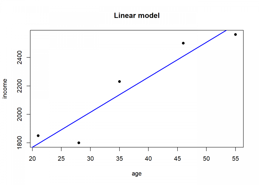
Linear modelling (e.g. correlation and linear regression) couldn’t be any easier, it is included in the core language:
age <- c(21, 46, 55, 35, 28)
income <- c(1850, 2500, 2560, 2230, 1800)
df <- data.frame(age, income) # create a data frame
df
##   age income
## 1  21   1850
## 2  46   2500
## 3  55   2560
## 4  35   2230
## 5  28   1800

cor(df) # correlation
##              age    income
## age    1.0000000 0.9464183
## income 0.9464183 1.0000000

LinReg <- lm(income ~ age, data = df) # income as a linear model of age
LinReg
##
## Call:
## lm(formula = income ~ age, data = df)
##
## Coefficients:
## (Intercept)          age
##     1279.37        24.56

summary(LinReg)
##
## Call:
## lm(formula = income ~ age, data = df)
##
## Residuals:
##       1       2       3       4       5
##   54.92   90.98  -70.04   91.12 -166.98
##
## Coefficients:
##             Estimate Std. Error t value Pr(>|t|)
## (Intercept) 1279.367    188.510   6.787  0.00654 **
## age           24.558      4.838   5.076  0.01477 *
## ---
## Signif. codes:  0 '***' 0.001 '**' 0.01 '*' 0.05 '.' 0.1 ' ' 1
##
## Residual standard error: 132.1 on 3 degrees of freedom
## Multiple R-squared:  0.8957, Adjusted R-squared:  0.8609
## F-statistic: 25.77 on 1 and 3 DF,  p-value: 0.01477

plot(df, pch = 16, main = "Linear model")
abline(LinReg, col = "blue", lwd = 2) # adding the regression line
You could directly use the model to make predictions:
pred_LinReg <- predict(LinReg, data.frame(age = seq(15, 70, 5)))
names(pred_LinReg) <- seq(15, 70, 5)
round(pred_LinReg, 2)
##      15      20      25      30      35      40      45      50      55
## 1647.73 1770.52 1893.31 2016.10 2138.88 2261.67 2384.46 2507.25 2630.04
##      60      65      70
## 2752.83 2875.61 2998.40
If you want to know more about the modelling process you can find it here: Learning Data Science: Modelling Basics.
Another strength of R is the huge number of add-on packages for all kinds of specialized tasks. For the grand finale of this introduction, we’re gonna get a little taste of machine learning. For that matter we install the OneR package from CRAN (the official package repository of R): Tools -> Install packages… -> type in “OneR” -> click “Install”.
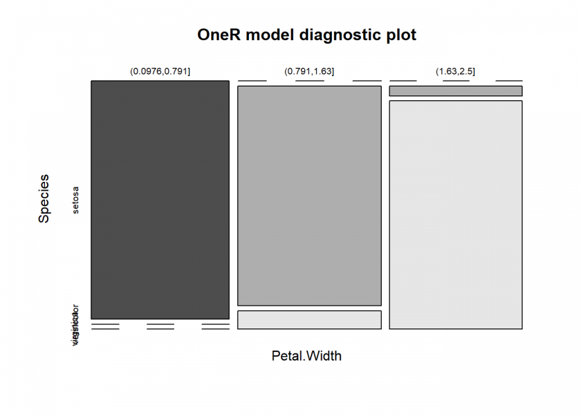
After that we build a simple model on the iris dataset to predict the Species column:
library(OneR) # load package
data <- optbin(Species ~., data = iris) # find optimal bins for numeric predictors
model <- OneR(data, verbose = TRUE) # build actual model
##
##     Attribute    Accuracy
## 1 * Petal.Width  96%
## 2   Petal.Length 95.33%
## 3   Sepal.Length 74.67%
## 4   Sepal.Width  55.33%
## ---
## Chosen attribute due to accuracy
## and ties method (if applicable): '*'

summary(model) # show rules
##
## Call:
## OneR.data.frame(x = data, verbose = TRUE)
##
## Rules:
## If Petal.Width = (0.0976,0.791] then Species = setosa
## If Petal.Width = (0.791,1.63]   then Species = versicolor
## If Petal.Width = (1.63,2.5]     then Species = virginica
##
## Accuracy:
## 144 of 150 instances classified correctly (96%)
##
## Contingency table:
##             Petal.Width
## Species      (0.0976,0.791] (0.791,1.63] (1.63,2.5] Sum
##   setosa               * 50            0          0  50
##   versicolor              0         * 48          2  50
##   virginica               0            4       * 46  50
##   Sum                    50           52         48 150
## ---
## Maximum in each column: '*'
##
## Pearson's Chi-squared test:
## X-squared = 266.35, df = 4, p-value < 2.2e-16

plot(model)
We’ll now see how well the model is doing:
prediction <- predict(model, data)
eval_model(prediction, data)
##
## Confusion matrix (absolute):
##             Actual
## Prediction   setosa versicolor virginica Sum
##   setosa         50          0         0  50
##   versicolor      0         48         4  52
##   virginica       0          2        46  48
##   Sum            50         50        50 150
##
## Confusion matrix (relative):
##             Actual
## Prediction   setosa versicolor virginica  Sum
##   setosa       0.33       0.00      0.00 0.33
##   versicolor   0.00       0.32      0.03 0.35
##   virginica    0.00       0.01      0.31 0.32
##   Sum          0.33       0.33      0.33 1.00
##
## Accuracy:
## 0.96 (144/150)
##
## Error rate:
## 0.04 (6/150)
##
## Error rate reduction (vs. base rate):
## 0.94 (p-value < 2.2e-16)
96% accuracy is not too bad, even for this simple dataset!
If you want to know more about the OneR package you can read the vignette: OneR – Establishing a New Baseline for Machine Learning Classification Models or find more examples in this blog: Category: OneR.

Well, and that’s it for the ultimate introduction to R – hopefully, you liked it and you learned something! Please share your first experiences with R in the comments and also if you miss something (I might add it in the future!) – Thank you for reading and stay tuned for more to come!
UPDATE September 24, 2021
I created a video for this post (in German):
no, no, no in R ultimate intro to ML is:
🙂
Thank you, p: I tried your code, and it gives the same accuracy as OneR but is much less interpretable. While OneR gives simple rules random forest is very much a black box.