

Have you ever thought about why the definition of a function in R is different from many other programming languages? The part that causes the biggest difficulties (especially for beginners of R) is that you state the name of the function at the beginning and use the assignment operator – as if functions were like any other data type, like vectors, matrices or data frames…
Congratulations! You just encountered one of the big ideas of functional programming: functions are indeed like any other data type, they are not special – or in programming lingo, functions are first-class members. Now, you might ask: So what? Well, there are many ramifications, for example, that you could use functions on other functions by using one function as an argument for another function. Sounds complicated?
In mathematics, most of you will be familiar with taking the derivative of a function. When you think about it you could say that you put one function into the derivative function (or operator) and get out another function!
In R there are many applications as well, let us go through a simple example step by step.
Let’s say I want to apply the mean function on the first four columns of the iris dataset. I could do the following:
mean(iris[ , 1])
## [1] 5.843333
mean(iris[ , 2])
## [1] 3.057333
mean(iris[ , 3])
## [1] 3.758
mean(iris[ , 4])
## [1] 1.199333

# or with pipe operator since R 4.1.0
iris[ , 1] |> mean()
## [1] 5.843333
iris[ , 2] |> mean()
## [1] 3.057333
iris[ , 3] |> mean()
## [1] 3.758
iris[ , 4] |> mean()
## [1] 1.199333
Quite tedious and not very elegant. Of course, we can use a for loop for that:
for (x in iris[1:4]) {
  print(mean(x))
}
## [1] 5.843333
## [1] 3.057333
## [1] 3.758
## [1] 1.199333
This works fine but there is an even more intuitive approach. Just look at the original task: “apply the mean function on the first four columns of the iris dataset” – so let us do just that:
apply(iris[1:4], 2, mean)
## Sepal.Length  Sepal.Width Petal.Length  Petal.Width
##     5.843333     3.057333     3.758000     1.199333
Wow, this is very concise and works perfectly (the 2 just stands for “go through the data column wise”, 1 would be for “row wise”). apply is called a “higher-order function” and we could use it with all kinds of other functions:
apply(iris[1:4], 2, sd)
## Sepal.Length  Sepal.Width Petal.Length  Petal.Width
##    0.8280661    0.4358663    1.7652982    0.7622377
apply(iris[1:4], 2, min)
## Sepal.Length  Sepal.Width Petal.Length  Petal.Width
##          4.3          2.0          1.0          0.1
apply(iris[1:4], 2, max)
## Sepal.Length  Sepal.Width Petal.Length  Petal.Width
##          7.9          4.4          6.9          2.5
You can also use user-defined functions:
midrange <- function(x) (min(x) + max(x)) / 2
apply(iris[1:4], 2, midrange)
## Sepal.Length  Sepal.Width Petal.Length  Petal.Width
##         6.10         3.20         3.95         1.30
We can even use new functions that are defined “on the fly” (or in functional programming lingo “anonymous functions”):
apply(iris[1:4], 2, function(x) (min(x) + max(x)) / 2)
## Sepal.Length  Sepal.Width Petal.Length  Petal.Width
##         6.10         3.20         3.95         1.30

apply(iris[1:4], 2, \(x) (min(x) + max(x)) / 2) # new shorthand syntax since R 4.1.0
## Sepal.Length  Sepal.Width Petal.Length  Petal.Width
##         6.10         3.20         3.95         1.30
Let us now switch to another inbuilt data set, the mtcars dataset with 11 different variables of 32 cars (if you want to find out more, please consult the documentation):
head(mtcars)
##                    mpg cyl disp  hp drat    wt  qsec vs am gear carb
## Mazda RX4         21.0   6  160 110 3.90 2.620 16.46  0  1    4    4
## Mazda RX4 Wag     21.0   6  160 110 3.90 2.875 17.02  0  1    4    4
## Datsun 710        22.8   4  108  93 3.85 2.320 18.61  1  1    4    1
## Hornet 4 Drive    21.4   6  258 110 3.08 3.215 19.44  1  0    3    1
## Hornet Sportabout 18.7   8  360 175 3.15 3.440 17.02  0  0    3    2
## Valiant           18.1   6  225 105 2.76 3.460 20.22  1  0    3    1
To see the power of higher-order functions let us create a (numeric) matrix with minimum, first quartile, median, mean, third quartile and maximum for all 11 columns of the mtcars dataset with just one command!
apply(mtcars, 2, summary)
##              mpg    cyl     disp       hp     drat      wt     qsec     vs      am   gear   carb
## Min.    10.40000 4.0000  71.1000  52.0000 2.760000 1.51300 14.50000 0.0000 0.00000 3.0000 1.0000
## 1st Qu. 15.42500 4.0000 120.8250  96.5000 3.080000 2.58125 16.89250 0.0000 0.00000 3.0000 2.0000
## Median  19.20000 6.0000 196.3000 123.0000 3.695000 3.32500 17.71000 0.0000 0.00000 4.0000 2.0000
## Mean    20.09062 6.1875 230.7219 146.6875 3.596563 3.21725 17.84875 0.4375 0.40625 3.6875 2.8125
## 3rd Qu. 22.80000 8.0000 326.0000 180.0000 3.920000 3.61000 18.90000 1.0000 1.00000 4.0000 4.0000
## Max.    33.90000 8.0000 472.0000 335.0000 4.930000 5.42400 22.90000 1.0000 1.00000 5.0000 8.0000
Wow, that was easy and the result is quite impressive, is it not!
Or if you want to perform a linear regression for all ten variables separately against mpg and want to get a table with all coefficients – there you go:
sapply(mtcars, function(x) round(coef(lm(mpg ~ x, data = mtcars)), 3))
##             mpg    cyl   disp     hp   drat     wt   qsec     vs     am  gear   carb
## (Intercept)   0 37.885 29.600 30.099 -7.525 37.285 -5.114 16.617 17.147 5.623 25.872
## x             1 -2.876 -0.041 -0.068  7.678 -5.344  1.412  7.940  7.245 3.923 -2.056
Here we used another higher-order function, sapply, together with an anonymous function. sapply goes through all the columns of a data frame (i.e. elements of a list) and tries to simplify the result (here your get back a nice matrix).
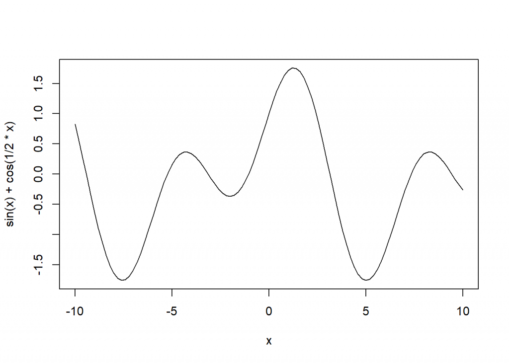
Often, you might not even have realized when you were using higher-order functions! I can tell you that it is quite a hassle in many programming languages to program a simple function plotter, i.e. a function which plots another function. In R it has already been done for you: you just use the higher-order function curve and give it the function you want to plot as an argument:
curve(sin(x) + cos(1/2 * x), -10, 10)
I want to give you one last example of another very helpful higher-order function (which not too many people know or use): by. It comes in very handy when you want to apply a function on different attributes split by a factor. So let’s say you want to get a summary of all the attributes of iris split by (!) species – here it comes:
by(iris[1:4], iris$Species, summary)
## iris$Species: setosa
##   Sepal.Length    Sepal.Width     Petal.Length    Petal.Width
##  Min.   :4.300   Min.   :2.300   Min.   :1.000   Min.   :0.100
##  1st Qu.:4.800   1st Qu.:3.200   1st Qu.:1.400   1st Qu.:0.200
##  Median :5.000   Median :3.400   Median :1.500   Median :0.200
##  Mean   :5.006   Mean   :3.428   Mean   :1.462   Mean   :0.246
##  3rd Qu.:5.200   3rd Qu.:3.675   3rd Qu.:1.575   3rd Qu.:0.300
##  Max.   :5.800   Max.   :4.400   Max.   :1.900   Max.   :0.600
## --------------------------------------------------------------
## iris$Species: versicolor
##   Sepal.Length    Sepal.Width     Petal.Length   Petal.Width
##  Min.   :4.900   Min.   :2.000   Min.   :3.00   Min.   :1.000
##  1st Qu.:5.600   1st Qu.:2.525   1st Qu.:4.00   1st Qu.:1.200
##  Median :5.900   Median :2.800   Median :4.35   Median :1.300
##  Mean   :5.936   Mean   :2.770   Mean   :4.26   Mean   :1.326
##  3rd Qu.:6.300   3rd Qu.:3.000   3rd Qu.:4.60   3rd Qu.:1.500
##  Max.   :7.000   Max.   :3.400   Max.   :5.10   Max.   :1.800
## --------------------------------------------------------------
## iris$Species: virginica
##   Sepal.Length    Sepal.Width     Petal.Length    Petal.Width
##  Min.   :4.900   Min.   :2.200   Min.   :4.500   Min.   :1.400
##  1st Qu.:6.225   1st Qu.:2.800   1st Qu.:5.100   1st Qu.:1.800
##  Median :6.500   Median :3.000   Median :5.550   Median :2.000
##  Mean   :6.588   Mean   :2.974   Mean   :5.552   Mean   :2.026
##  3rd Qu.:6.900   3rd Qu.:3.175   3rd Qu.:5.875   3rd Qu.:2.300
##  Max.   :7.900   Max.   :3.800   Max.   :6.900   Max.   :2.500
This was just a very shy look at this huge topic. There are very powerful higher-order functions in R, like lapppy, aggregate, replicate (very handy for numerical simulations) and many more. A good overview can be found in the answers of this question: Grouping functions (tapply, by, aggregate) and the *apply family (my answer there is on the rather illusive sweep function: sweep).
For some reason, people tend to confuse higher-order functions with recursive functions but that is the topic of another post, so stay tuned…
UPDATE February 19, 2019
The post on recursion is now online:
To understand Recursion you have to understand Recursion….
vonJD,
Thanks for the blog posts. I really appreciate your explanations of “apply” and “oneR”. You write in a perfect style for quick comprehension. It is a gift to be able to teach well, and you seem to have it. Happy holidays!
~Jeff
Wow, thank you very much for the great feedback, Jeff!
R is such a wonderful, versatile language with so many different areas of application and I have many fun projects up my sleeve – so stay tuned 🙂
Happy holidays to you too!
best
h