Will I get my Money back? Credit Scoring with OneR

More and more decisions by banks on who gets a loan are being made by artificial intelligence. The terms being used are credit scoring and credit decisioning.

They base their decisions on models whether the customer will pay back the loan or will default, i.e. determine their creditworthiness. If you want to learn how to build such a model in R yourself (with the latest R ≥ 4.1.0 syntax as a bonus), read on!

As always we need data to build our model. In this case we will use credit scoring data from a kaggle competition: Give Me Some Credit (we will use the file cs-training.csv, you might have to register to download it).

The goal is to predict whether somebody will experience financial distress in the next two years, the full list of variables includes:

• Serious delinquency in 2 years (SeriousDlqin2yrs)
• Revolving Utilization Of Unsecured Lines
• Age of borrower in years
• Number Of Time 30–59 Days Past Due Not Worse
• Debt Ratio
• Monthly Income
• Number Of Open Credit Lines And Loans
• Number Of Times 90 Days Late
• Number of Real Estate Loans Or Lines
• Number Of Time 60–89 Days Past Due Not Worse
• Number of Dependents

We start by reading the data into R and inspecting it:

cs <- read.csv("data/cs-training.csv")
data <- cs[ , -1]
str(data)
## 'data.frame':    150000 obs. of  11 variables:
##  $ SeriousDlqin2yrs                    : int  1 0 0 0 0 0 0 0 0 0 ...
##  $ RevolvingUtilizationOfUnsecuredLines: num  0.766 0.957 0.658 0.234 0.907 ...
##  $ age                                 : int  45 40 38 30 49 74 57 39 27 57 ...
##  $ NumberOfTime30.59DaysPastDueNotWorse: int  2 0 1 0 1 0 0 0 0 0 ...
##  $ DebtRatio                           : num  0.803 0.1219 0.0851 0.036 0.0249 ...
##  $ MonthlyIncome                       : int  9120 2600 3042 3300 63588 3500 NA 3500 NA 23684 ...
##  $ NumberOfOpenCreditLinesAndLoans     : int  13 4 2 5 7 3 8 8 2 9 ...
##  $ NumberOfTimes90DaysLate             : int  0 0 1 0 0 0 0 0 0 0 ...
##  $ NumberRealEstateLoansOrLines        : int  6 0 0 0 1 1 3 0 0 4 ...
##  $ NumberOfTime60.89DaysPastDueNotWorse: int  0 0 0 0 0 0 0 0 0 0 ...
##  $ NumberOfDependents                  : int  2 1 0 0 0 1 0 0 NA 2 ...

We see that we have 150,000 observations altogether, which we split randomly into a training (80%) and a test (20%) set:

set.seed(3141) # for reproducibility
random <- sample(1:nrow(data), 0.8 * nrow(data))
data_train <- data[random, ]
data_test <- data[-random, ]

We will build our model with the OneR package (on CRAN, for more posts on this package see Category: OneR). I will use the new native pipe operator |>, in combination with the new shorthand syntax \(x) for anonymous functions, to build the model. You will need at least R version 4.1.0 to run the code. For comparison, I include the traditional form in the comments above the new syntax:

library(OneR)

# same as 'model <- OneR(optbin(SeriousDlqin2yrs ~., data = data_train))'
model <- data_train |> {\(x) optbin(SeriousDlqin2yrs ~., data = x)}() |> OneR()
## Warning in optbin.data.frame(x = data, method = method, na.omit = na.omit):
## target is numeric
## Warning in optbin.data.frame(x = data, method = method, na.omit = na.omit):
## 23698 instance(s) removed due to missing values

# same as summary(model)
model |> summary()
## 
## Call:
## OneR.data.frame(x = {
##     function(x) optbin(SeriousDlqin2yrs ~ ., data = x)
## }(data_train))
## 
## Rules:
## If NumberOfTimes90DaysLate = (-0.098,1.6] then SeriousDlqin2yrs = 0
## If NumberOfTimes90DaysLate = (1.6,98.1]   then SeriousDlqin2yrs = 1
## 
## Accuracy:
## 89774 of 96302 instances classified correctly (93.22%)
## 
## Contingency table:
##                 NumberOfTimes90DaysLate
## SeriousDlqin2yrs (-0.098,1.6] (1.6,98.1]   Sum
##              0        * 88719        863 89582
##              1           5665     * 1055  6720
##              Sum        94384       1918 96302
## ---
## Maximum in each column: '*'
## 
## Pearson's Chi-squared test:
## X-squared = 6946.5, df = 1, p-value < 2.2e-16

# same as plot(model)
model |> plot()

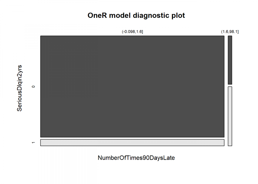
We see that the data are extremely unbalanced, which is quite normal for credit scoring data because most customers (thankfully!) pay back their loans. Still, OneR was able to find a simple rule: If the borrower has been 90 days or more past due more than once chances are that (s)he will default on the loan. Let us see how well this model fares with the test set:

# same as 'eval_model(prediction = predict(model, data_test), actual = data_test$SeriousDlqin2yrs)'
data_test |> {\(x) eval_model(prediction = predict(model, x), actual = x$SeriousDlqin2yrs)}()
## 
## Confusion matrix (absolute):
##           Actual
## Prediction     0     1   Sum
##        0   27745  1621 29366
##        1     269   365   634
##        Sum 28014  1986 30000
## 
## Confusion matrix (relative):
##           Actual
## Prediction    0    1  Sum
##        0   0.92 0.05 0.98
##        1   0.01 0.01 0.02
##        Sum 0.93 0.07 1.00
## 
## Accuracy:
## 0.937 (28110/30000)
## 
## Error rate:
## 0.063 (1890/30000)
## 
## Error rate reduction (vs. base rate):
## 0.0483 (p-value = 0.01284)

The accuracy of the model of nearly 94% is quite good. One important point to keep in mind though: because of the extreme imbalance of the data this accuracy is a little bit misleading. Yet the last line of the output above (error rate reduction with p < 0.05) tells us that despite this imbalance the model really is able to give better predictions than a naive approach (if you want to know more about this please consult: ZeroR: The Simplest Possible Classifier… or: Why High Accuracy can be Misleading).

Anyway, it is way better than this use case from “DataRobot” on the same dataset which had an accuracy of just about 77%: Predicting financial delinquency using credit scoring data. That model is way more complex, less interpretable, needed more tweaking, and was built using proprietary software on a 72 core private cloud for about five hours. We built our way better model out of the box with the freely available OneR-package on a 10-year-old computer within seconds!