Learning Machines proudly presents a fascinating guest post by decision and risk analyst Robert D. Brown III with a great application of R in the business and especially startup-arena! I encourage you to visit his blog too: Thales’ Press. Have fun!
Introduction
While Excel remains the tool of choice among analysts for business case analysis, presumably because of its low barrier to entry and ease of use, it nonetheless continues to be the source of many vexing and disastrous errors. As the research from Panko and others have revealed, the source of these errors arise in part for the following reasons:
- Analysts continue in a persistent lack of QA standards and practices to ensure that spreadsheets are as error free as possible.
- Cell referencing and replicating formulas across relevant dimensions propagate errors at exponential rates.
- Effective auditing gets obscured because formulas’ conceptual meanings are difficult to interpret from formulas constructed from grid coordinates.
To suggest a means to remedy that situation, in the spring of 2018, I published Business Case Analysis with R: Simulation Tutorials to Support Complex Business Decisions (BCAwR). I also wanted to showcase how the popular programming language R could be employed to evaluate business case opportunities that are fraught with uncertainty nor supported by an abundance of well structured, pedigreed, and relevant data, a situation that plagues just about all business decisions faced in the real world. BCAwR takes the reader through the process of analyzing a rather complex commercial investment problem of bringing a chemical processing plant on line. For my post here, I will present a simplified model to give a preview of the contents of the book. I will also provide a little surprise at the end that I hope will contribute to bridging the efforts of the decision and data science communities.
But before we delve into any coding or quantitative activity related to analysis of any business case, we ought to thoroughly frame our problem by narrowing the scope of our inquiry to the appropriate level for the context of the problem at hand, identifying the goals and objectives we want to achieve when we eventually commit to action, partitioning the set of actionable decision we can make to achieve our goals, and creating an inventory of the influences and relationships that connect decisions and uncertainties to the measures of success. Although we will look at a much more simplified business problem here, a little framing will still serve us well.
Imagine that we are considering investing in a project that solves a particular market problem with the ultimate desire to generate a financial return to our organization. We identify three possible strategic pathways to compare for the investment, each with a different level of capital commitment required to address certain nuances of the market problem. Each (1) investment, in turn, will generate (2) an initial post investment net cash flow, (3) a peak cash flow, and varying durations of (4) time to reach the peak from the initial cash flow.
To complicate the matter, for each strategy, we do not know the precise quantitative value of the four parameters that characterize the potential cash flow. For this reason, when we evaluate the three strategies, we will employ a Monte Carlo simulation approach that samples a large number of potential realizations for each parameter from probability distributions. With these ideas in mind, we can now set up the coding to handle the simulation problem.
library(leonRdo) # https://www.incitedecisiontech.com/packages/packages.html
library(tidyverse) # (on CRAN)
# Set the simulation seed.
set.seed(42)

# The number of simulation runs per uncertain variable.
trials <- 1000

# The time frame across which our cash flow simulation will run.
# The initial investment will occur in year 0.
year <- 0:15

# The weighted average cost of capital without any additional risk premium.
discount.rate <- 0.1

# The distinctive capital allocation strategic decisions.
strategy <- c("Strategy 1", "Strategy 2", "Strategy 3")
R employs simple Monte Carlo techniques, which doesn’t typically yield stable means for result distributions until many thousands of trials are used. However, When developing a model like this, I suggest setting the trials to 50-100 to make sure that the logic is running correctly in short responsive time frames. Then, when you’re ready to produce real results, change the values to greater than 10,000. Given that Monte Carlo in R is noisy even for reasonably large samples (~1000) and for different seed settings, I recently developed the leonRdo package (R Packages: leonRdo & inteRest) to provide a median Latin hypercube approach to sampling that produces much more stable means with approximately 1/10th the number of trials regardless of the seed value used.
In this particular showcase discussion, I have included the tidyverse package (on CRAN) to help with data manipulation and graphing. In the original BCAwR, I based all the code on base R so that readers new to R and simulation could focus more on learning the key principles over the idiosyncratic syntax of secondary packages.
The set.seed() function ensures that we will produce the same sample trial set on each run of our model. This will help us debug problems as we develop code. Eventually as others might interact with our code, they will be able to observe the same set of results we work with. Later, we can reset the seed to other values to make sure that our inferences on a given set of trials remain consistent on a different trial set.
Model Functions
Next, we need to declare some important functions that we will call in our model. The first is a function that provides an analytic solution to the differential equation that relates the proportional absorption of an entity into a fixed environment. This ramp up function takes as parameters the amount of time Tp required to go from, say, Y = 1% absorption to Y = 99% across Time. We will use this function to model the growth of our cash flow over the year index.
# Ramp up function.
calcRampUp <- function(Y0, Time, Tp) {
  # Y0 = initial absorption
  # Time = time index
  # tp = time to Y = 1 - Y0, the time to peak.
  Y <- 1 / (1 + (Y0 / (1 - Y0)) ^ (2 * (Time - 1) / (Tp - 1) - 1))
  return(Y)
}
The second function we need is the actual business model we want to represent. The business model logic will remain fixed across strategies, and the results will vary only on the basis of the strategy conditional parameters we supply. By “functionalizing” our model, we can iterate the entire model over variable ranges to understand the sensitivity of the output function to those variables, as we shall later see. Please note, this is a toy model we are using for illustration purposes only. BCAwR demonstrates a much more complex consideration for the implementation of a chemical processing plant.
# Business model cash flow.
calcCashFlow <- function(I, SCF, PCF, YP, Y) {
  # I = initial investment
  # SCF = starting cash flow
  # PCF = peak cash flow
  # YP = year of peak cash flow
  # Y = year index
  cf <- (Y == 0) * (-I) +
    (Y > 0) * (SCF + (PCF - SCF) * calcRampUp(0.01, Y, YP))
  return(cf)
}
The last function we will employ is the net present value (NPV) function that we will apply to the individual trial results of the cash flow simulation across strategies.
# The net present value of the cash flow function.
calcNPV <- function(CF, Y, DR) {
  # CF = cash flow vector
  # Y = year index
  # DR = discount rate
  npv <- sum(CF / (1 + DR) ^ Y)
  return(npv)
}
Initialize Simulation Trial Samples
Our next task is to create trial samples for the business model cash flow function parameters for the three project strategy investments. For this particular example, I have chosen to use canonical distributions as if their parameters were based on empirical or historical data and to utilize a simple method for generating trials. However, typically I would use a combination of both empirical data and subject matter expert guidance reflected as cumulative probabilities across the range of the assessed variables’ potential values. I explain how to take this latter approach in greater detail in Section III of BCAwR.
investment1 <-
  rlnorm_mlhs(n = trials,
         meanlog = log(800),
         sdlog = log(1 + 200 / 800))
investment2 <-
  rlnorm_mlhs(n = trials,
         meanlog = log(700),
         sdlog = log(1 + 50 / 700))
investment3 <-
  rlnorm_mlhs(n = trials,
         meanlog = log(1000),
         sdlog = log(1 + 150 / 1000))

start.cash.flow1 <- rnorm_mlhs(n = trials, mean = -100, sd = 20)
start.cash.flow2 <- rnorm_mlhs(n = trials, mean = -90, sd = 5)
start.cash.flow3 <- rnorm_mlhs(n = trials, mean = -120, sd = 15)

peak.cash.flow1 <- rnorm_mlhs(n = trials, mean = 300, sd = 20)
peak.cash.flow2 <- rnorm_mlhs(n = trials, mean = 280, sd = 5)
peak.cash.flow3 <- rnorm_mlhs(n = trials, mean = 375, sd = 15)

yr.peak1 <- rnorm_mlhs(n = trials, mean = 8.5, sd = 0.75)
yr.peak2 <- rnorm_mlhs(n = trials, mean = 10, sd = 0.85)
yr.peak3 <- rnorm_mlhs(n = trials, mean = 11, sd = 1)

# Store the business model parameter samples in a list of data frames.
proj.data <-
  list(
    investment = data.frame(investment1, investment2, investment3),
    start.cash.flow = data.frame(start.cash.flow1, start.cash.flow2, start.cash.flow3),
    peak.cash.flow = data.frame(peak.cash.flow1, peak.cash.flow2, peak.cash.flow3),
    yr.peak = data.frame(yr.peak1, yr.peak2, yr.peak3)
  )
Model Results
For each strategy, we apply the samples from each parameter to the business model cash flow function. This will result in a list of cash flows for the three project strategies. For each strategy, there will be as many cash flows as defined by trials, and each cash flow trial will be as long as the year index. We can use the lapply() and sapply() functions to avoid using for loops [see also Learning R: A gentle introduction to higher-order functions].
proj.cf <- lapply(1:length(strategy), function(s) {
  sapply(1:trials, function(t) {
    calcCashFlow(
      I = proj.data$investment[[s]][t],
      SCF = proj.data$start.cash.flow[[s]][t],
      PCF = proj.data$peak.cash.flow[[s]][t],
      YP = proj.data$yr.peak[[s]][t],
      Y = year
    )
  })
})
names(proj.cf) <- strategy
By running the first five trials of Strategy 1, we can see what the cash flows look like.
head(round(proj.cf[[1]][, 1:5], digits = 1), n=length(year))
##         [,1]   [,2]   [,3]   [,4]   [,5]
##  [1,] -852.7 -852.2 -766.7 -974.3 -912.6
##  [2,]  -85.8 -103.1 -117.2 -116.1  -88.1
##  [3,]  -77.8  -93.6 -107.3 -106.9  -79.9
##  [4,]  -55.3  -64.3  -76.7  -79.9  -57.1
##  [5,]    0.0    9.4    0.2  -13.1   -1.6
##  [6,]   98.0  128.7  123.7  102.2   97.9
##  [7,]  201.5  230.2  227.2  215.6  206.8
##  [8,]  265.3  279.2  276.2  279.8  276.9
##  [9,]  292.5  296.5  293.3  305.3  308.0
## [10,]  302.3  301.8  298.5  314.1  319.5
## [11,]  305.6  303.4  300.1  316.9  323.5
## [12,]  306.7  303.9  300.5  317.8  324.8
## [13,]  307.1  304.1  300.7  318.1  325.2
## [14,]  307.2  304.1  300.7  318.2  325.4
## [15,]  307.2  304.1  300.7  318.2  325.4
## [16,]  307.2  304.1  300.7  318.2  325.5
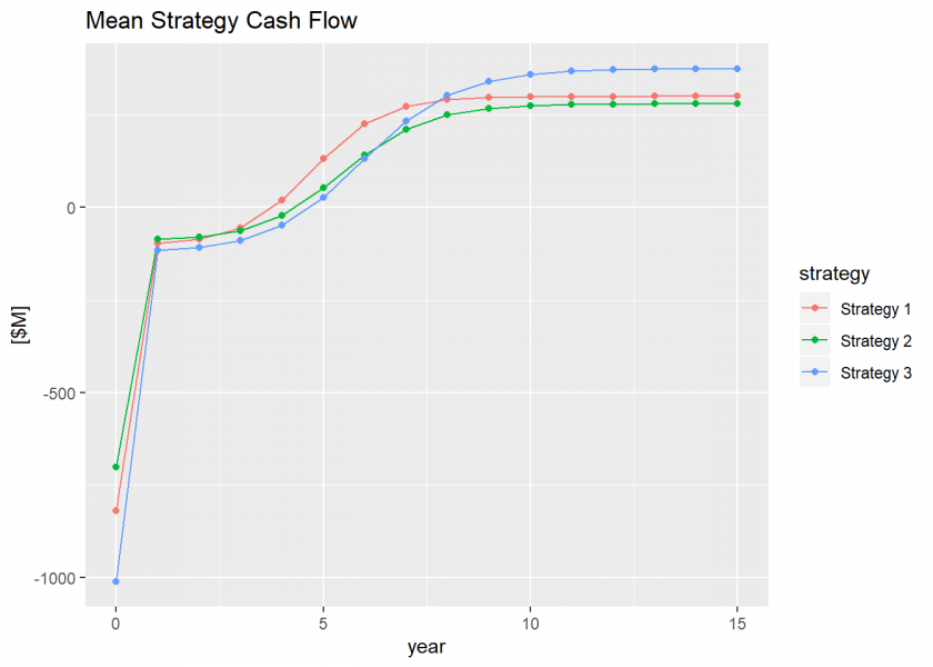
We can calculate some summary results for the cash flows for each strategy and plot them. First, we might like to plot the mean cash flow over time.
proj.cf.mean <- as.data.frame(lapply(strategy, function(s) {
  rowMeans(proj.cf[[s]])
}))
names(proj.cf.mean) <- strategy
proj.cf.mean <- cbind(year, proj.cf.mean)

# Plot the mean strategy cash flows.
gg.mean.cf <-
  ggplot(gather(proj.cf.mean, "strategy", "mean", -year)) +
  geom_line(aes(x = year, y = mean, color = strategy)) +
  geom_point(aes(x = year, y = mean, color = strategy)) +
  labs(title = "Mean Strategy Cash Flow",
       y = "[$M]")
plot(gg.mean.cf)

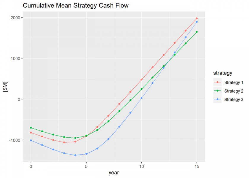
Then we can calculate the cumulative mean cash flow and plot that for each strategy, too.
proj.ccf.mean <- proj.cf.mean %>%
  mutate_at(vars(strategy), list(~ cumsum(.)))

# Plot the cumulative mean strategy cash flows.
gg.mean.ccf <-
  ggplot(gather(proj.ccf.mean, "strategy", "mean", -year)) +
  geom_line(aes(x = year, y = mean, color = strategy)) +
  geom_point(aes(x = year, y = mean, color = strategy)) +
  labs(title = "Cumulative Mean Strategy Cash Flow",
       y = "[$M]")
plot(gg.mean.ccf)

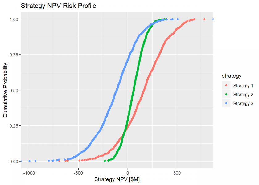
Now we can observe the risk profile of the cash flows by calculating the trial NPVs of the cash flows.
proj.npv <- as.data.frame(lapply(1:length(strategy), function(s) {
  sapply(1:trials, function(t) {
    calcNPV(CF = proj.cf[[s]][, t],
            Y = year,
            DR = discount.rate)
  })
}))
names(proj.npv) <- strategy

# Plot the CDF of the strategies' sample NPVs.
gg.ecdf <-
  ggplot(gather(proj.npv, "strategy", "NPV"), aes(x = NPV, color = strategy)) +
  stat_ecdf(geom = "point") +
  labs(title = "Strategy NPV Risk Profile",
       x = "Strategy NPV [$M]",
       y = "Cumulative Probability")
plot(gg.ecdf)

And we can calculate the mean NPV of the cash flows.
proj.npv.mean <- round(colMeans(proj.npv), digits = 1)
print(proj.npv.mean)
## Strategy 1 Strategy 2 Strategy 3
##      157.4       59.3     -123.6
The first observation we make about the risk profiles of the strategies is that we can dismiss Strategy 3 immediately because it presents negative mean NPV, the probability that it produces a negative economic value is ~75% (i.e., the probability(NPV<=0) = 0.75), and practically none of its trials present any opportunity for dominance over any other strategy.
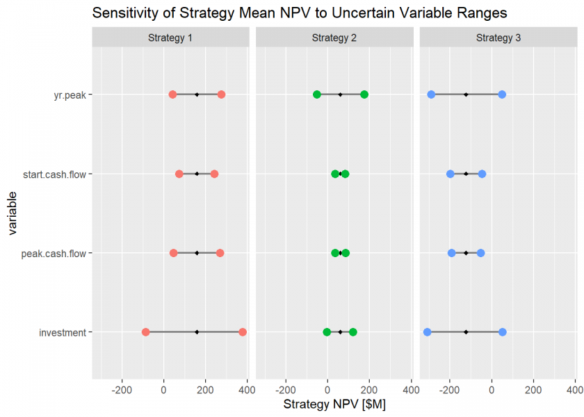
When we observe the relative volatility and dominance of the remaining strategies, we realize that we face a bit of ambiguity about how to choose the best pathway forward. Strategy 1 exhibits the best overall mean NPV, but it does so with the greatest relative volatility. While Strategy 2 exhibits approximately the same risk of failure (~25%) as Strategy 1 (~27%), it also exhibits the least maximum exposure and relative volatility. To reduce the ambiguity of choosing, we might like to know which uncertainty, due to the overall quality of the information we possess about it, contributes most to switching dominance from Strategy 1 over Strategy 2. Knowing which uncertainty our strategy values are most sensitive to gives us the ability to stop worrying about the other uncertainties for the purpose of choosing clearly and focus only on improving our understanding of those that matter most.
To accomplish that latter feat, we run our functionalized model to test the sensitivity of the strategy means to the 80th percentile range in each of the variables. We start by initializing the lists to hold the sensitivity responses.
data.temp <- proj.data
proj.npv.sens <- list(p10 = proj.data,
                      p90 = proj.data)
d <- data.frame(0, 0, 0)
dd <-
  list(
    investment = d,
    start.cash.flow = d,
    peak.cash.flow = d,
    yr.peak = d
  )
proj.npv.sens.mean <- list(p10 = dd,
                           p90 = dd)
We calculate the sensitivity of the strategies’ mean NPVs by fixing each variable to its p10 and p90 quantile values sequentially while all the other variables run according to their defined variation. The result is a chart that shows how sensitive we might be to changing our decision to pursue the best strategy over the next best strategy on the outcome of a given uncertainty.
p1090 <- c(0.1, 0.9)
for (q in 1:length(p1090)) {
  for (v in 1:length(proj.data)) {
    for (s in 1:length(strategy)) {
      data.temp[[v]][s] <-
        rep(quantile(unlist(proj.data[[v]][s]), probs = p1090[q]), trials)
      for (t in 1:trials) {
        proj.npv.sens[[q]][[v]][t, s] <- calcNPV(
          CF = calcCashFlow(
            I = data.temp$investment[[s]][t],
            SCF = data.temp$start.cash.flow[[s]][t],
            PCF = data.temp$peak.cash.flow[[s]][t],
            YP = data.temp$yr.peak[[s]][t],
            Y = year
          ),
          Y = year,
          DR = discount.rate
        )
      }
      proj.npv.sens.mean[[q]][[v]][s] <-
        mean(proj.npv.sens[[q]][[v]][, s])
      data.temp <- proj.data
    }
  }
}

# Recast the sensitivity values to a form that can be plotted.
variable.names <-
  c("investment", "start.cash.flow", "peak.cash.flow", "yr.peak")
proj.npv.sens.mean2 <- as.data.frame(sapply(1:length(p1090), function(q) {
  sapply(1:length(proj.data), function(v) {
    sapply(1:length(strategy), function(s) {
      proj.npv.sens.mean[[q]][[v]][[s]]
    })
  })
})) %>%
  rename(p10 = V1,
         p90 = V2) %>%
  mutate(
    variable = rep(variable.names, each = length(strategy)),
    strategy = rep(strategy, times = length(proj.data)),
    strategy.mean = rep(t(proj.npv.mean), times = length(proj.data))
  ) %>%
  select(variable, strategy, strategy.mean, p10, p90)

gg.sens <-
  ggplot(proj.npv.sens.mean2,
         aes(
           x = variable,
           y = p10,
           yend = p90,
           color = strategy
         )) +
  geom_segment(aes(
    x = variable,
    xend = variable,
    y = p10,
    yend = p90
  ),
  color = "gray50",
  size = 0.75) +
  geom_point(
    aes(x = variable, y = strategy.mean, color = strategy),
    size = 1,
    color = "black",
    fill = "black",
    shape = 23
  ) +
  geom_point(
    aes(x = variable, y = p90),
    size = 3) +
  geom_point(
    aes(x = variable, y = p10),
    size = 3) +
  labs(title = "Sensitivity of Strategy Mean NPV to Uncertain Variable Ranges",
       y = "Strategy NPV [$M]") +
  coord_flip() +
  theme(legend.position = "none") +
  facet_wrap(~ strategy)
plot(gg.sens)

This sensitivity chart is valuable not only to the decision analyst, but to the data analyst as well for this one simple reason: now that we know which uncertainties potentially exposes us to the greatest risk or reward, we can calculate the value of information on those uncertainties. This value of information represents the rational maximum budget we should allocate to acquire better data and insight on those uncertainties. While a typical business case analysis of sufficient complexity may contain 10-100 uncertainties, we should focus our research budget only on those that are critical to making a decision. This simple “stopping function” helps us ensure that our data science resources are allocated properly and most efficiently. Section IV of BCAwR provides a means to calculate the value of information on continuous variables like the ones we have utilized in our example here.
Conclusion
Business decision analysts can definitely use R effectively to conduct many of the business case analyses in a more transparent and less error prone environment than their current tools typically allow, especially through the use of clearly named variables that array abstract and the use of functionalized structural models. However, the real power that R provides is the means to simulate information when high quality, large scale data may be scarce, infeasible, or impossible to obtain. Then, by using such concepts as value of information, data scientists can be called upon to refine the quality of information on those critical uncertainties that may frustrate success when commitment to action turns into real decisions. I hope the simple example presented here inspires you to learn more about it.

Thank u for sharing this is very important…
Thank you for your feedback!
Great post! this is very useful and informative…