We already covered the so-called Accuracy-Interpretability Trade-Off which states that oftentimes the more accurate the results of an AI are the harder it is to interpret how it arrived at its conclusions (see also: Learning Data Science: Predicting Income Brackets).
This is especially true for Neural Networks: while often delivering outstanding results, they are basically black boxes and notoriously hard to interpret (see also: Understanding the Magic of Neural Networks).
There is a new hot area of research to make black-box models interpretable, called Explainable Artificial Intelligence (XAI), if you want to gain some intuition on one such approach (called LIME), read on!
Before we dive right into it it is important to point out when and why you would need interpretability of an AI. While it might be a desirable goal in itself it is not necessary in many fields, at least not for users of an AI, e.g. with text translation, character and speech recognition it is not that important why they do what they do but simply that they work.
In other areas, like medical applications (determining whether tissue is malignant), financial applications (granting a loan to a customer) or applications in the criminal-justice system (gauging the risk of recidivism) it is of the utmost importance (and sometimes even required by law) to know why the machine arrived at its conclusions.
One approach to make AI models explainable is called LIME for Local Interpretable Model-Agnostic Explanations. There is already a lot in this name!
- First, you are able to make any (!) model interpretable (so not only neural networks).
- Second, the explanation is always on a specific case, so the method tries to explain e.g. why this specific customer wasn’t approved for a loan but no general explanations, what is important to get a loan, will be given.
- Third, and now we are getting at the heart of the method already, it approximates the complex, unintelligible model with a linear model.
This idea is, in my opinion, quite sexy because it has its equivalent in calculus: if you zoom in deep enough you can build most (even very complicated) function out of linear building blocks. This is what LIME basically does!
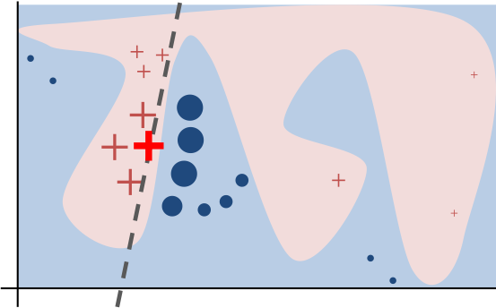
To gain some intuition we will use a very similar method and compare that with the results of LIME. We will even use the same illustrative picture used in the original paper (“Why Should I Trust You?”: Explaining the Predictions of Any Classifier) and create a toy-example out of it:

The paper explains (p. 4):
Toy example to present intuition for LIME. The black-box model’s complex decision function f (unknown to LIME) is represented by the blue/pink background, which cannot be approximated well by a linear model. The bold red cross is the instance being explained. LIME samples instances, gets predictions using f, and weighs them by the proximity to the instance being explained (represented here by size). The dashed line is the learned explanation that is locally (but not globally) faithful.
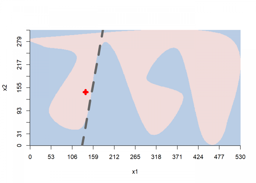
We are now taking this picture as our actual black-box model and approximate the decision boundary linearly. We do this by using logistic regression (see also: Learning Data Science: The Supermarket knows you are pregnant before your Dad does). LIME itself uses LASSO regression (see also: Cambridge Analytica: Microtargeting or How to catch voters with the LASSO).
Another thing is that we don’t weigh instances by proximity but randomly create more data points that are nearer to the respective case (by sampling from a multivariate normal distribution), yet the idea is the same.
Now we are ready to get started (you can find the prepared image here lime2.jpg, the packages jpeg and lime are on CRAN):
library(jpeg)
library(lime)

img <- readJPEG("pics/lime2.jpg") # adjust path
border_col <- mean(img[ , , 1])
model <- ifelse(img[ , , 1] < border_col, 0, 1)
image(model, axes = FALSE, xlab = "x1", ylab = "x2", col = c("#B9CDE5", "#F1DCDB"))
axis(1, at = seq(0, 1, .1), labels = seq(0, nrow(model), round(nrow(model)/10)))
axis(2, at = seq(0, 1, .1), labels = seq(0, ncol(model), round(ncol(model)/10)))

# some S3 magic
class(model) <- "black_box"
predict.black_box <- function(model, newdata, type = "prob") {
  newdata <- as.matrix(newdata)
  apply(newdata, 1, function(x) model[x[1], x[2]])
}

# the case to be analyzed
x1 <- 140; x2 <- 145
points(x1/nrow(model), x2/ncol(model), pch = 3, lwd = 6, col = "red")
predict(model, cbind(x1, x2))
## [1] 1

# approximate locally by logistic regression
set.seed(123)
x1_prox <- round(rnorm(100, x1, 18))
x2_prox <- round(rnorm(100, x2, 18))
data <- cbind(x1_prox, x2_prox)
df <- cbind.data.frame(y = predict(model, data), data)

logreg <- glm(y ~ ., data = df, family = binomial)
## Warning: glm.fit: algorithm did not converge
## Warning: glm.fit: fitted probabilities numerically 0 or 1 occurred

summary(logreg)
##
## Call:
## glm(formula = y ~ ., family = binomial, data = df)
##
## Deviance Residuals:
##        Min          1Q      Median          3Q         Max
## -6.423e-04   2.000e-08   2.000e-08   2.000e-08   5.100e-04
##
## Coefficients:
##              Estimate Std. Error z value Pr(>|z|)
## (Intercept)  12378.05  735651.83   0.017    0.987
## x1_prox        -94.11    5606.33  -0.017    0.987
## x2_prox         15.67     952.47   0.016    0.987
##
## (Dispersion parameter for binomial family taken to be 1)
##
##     Null deviance: 1.0279e+02  on 99  degrees of freedom
## Residual deviance: 8.5369e-07  on 97  degrees of freedom
## AIC: 6
##
## Number of Fisher Scoring iterations: 25

slope <- -coef(logreg)[2] / coef(logreg)[3]
intercept <- -coef(logreg)[1] / coef(logreg)[3]
segments(0, intercept/ncol(model), 1, (intercept + nrow(model) * slope)/ncol(model), lty = 2, lwd = 6, col = "grey40")

Here we can clearly see the locally approximated linear decision boundary. Now for the interpretation of the coefficients of the linear model:
# interpretation
barplot(coef(logreg)[3:2], horiz = TRUE, col = ifelse(coef(logreg)[3:2] < 0, "firebrick", "steelblue"), border = NA, xlab = "Weight", ylab = "Feature",  main = "Coefficients of linear model")
legend("bottom", horiz = TRUE, c("Supports", "Contradicts"), fill = c("steelblue", "firebrick"))

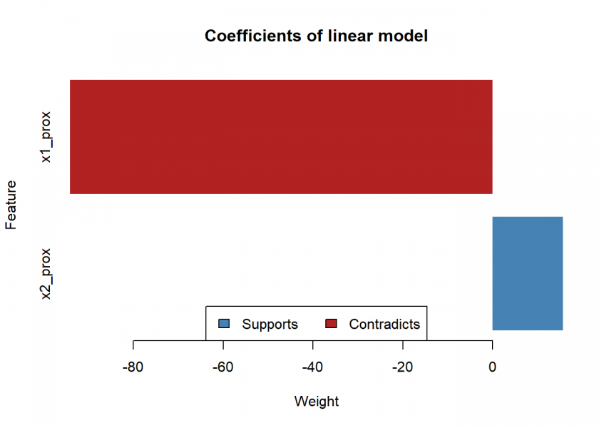
The bar chart can be interpreted like so: attribute x1 has a strong negative influence on the resulting class (i.e. when you increase it the class will quickly change), while attribute x2 has a comparatively mild positive influence (i.e. when you increase it the class won’t change but the model will get even more confident, but only mildly so). This interpretation can also readily be understood when looking at the decision boundary above.
We are now going to compare this with the original LIME method:
# compare with original lime
data <- expand.grid(1:nrow(model), 1:ncol(model))
colnames(data) <- c("x1", "x2")
train <- data.frame(data, y = predict(model, data))

explainer <- lime(train, model)
## Warning: y does not contain enough variance to use quantile binning. Using
## standard binning instead.

model_type.black_box <- function(x, ...) 'classification'
explanation <- explain(data.frame(x1 = 140, x2 = 145), explainer, n_labels = 1, n_features = 2)
explanation
## # A tibble: 2 x 13
##   model_type case  label label_prob model_r2 model_intercept
##   <chr>      <chr> <chr>      <dbl>    <dbl>           <dbl>
## 1 classific~ 1     p              1   0.0515           0.511
## 2 classific~ 1     p              1   0.0515           0.511
## # ... with 7 more variables: model_prediction <dbl>, feature <chr>,
## #   feature_value <dbl>, feature_weight <dbl>, feature_desc <chr>,
## #   data <list>, prediction <list>

plot_features(explanation, ncol = 1)

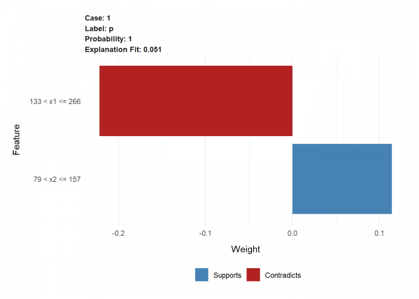
While the results are not a full match (because of the slightly different approach taken here) the direction and ratio of the magnitude are very similar.
All in all, I think LIME is a very powerful and intuitive method to whiten any black-box model and XAI will be one of the most important and relevant research areas in machine learning and artificial intelligence in the future!

Hi,
I wanted to ask you some questions about your post “Cambridge Analytica:
Microtargeting or How to catch voters with the LASSO October 8, 2019.
Would you mind sharing your email?
Thanks
You have provided yours, so I can contact you if you like… yet, would you mind asking your questions in the comment section below that post?
You can also get in touch with me here: https://blog.ephorie.de/about
ReLU as literal switch makes neural nets quite explainable:
https://ai462qqq.blogspot.com/2019/11/artificial-neural-networks.html
Could you please explain how this should work? I don’t see how this could help.
ReLU as a switch:
On: f(x)=z (connect.)
Off: f(x)=0 (disconnect.)
An audio source switch on an audio amplifier may have only 2 states, ‘on’ and ‘off.’
When ‘on’ it allows through a complicated audio signal. You can understand ReLU in a similar way.
The dot product (weighted sum) of a number of dot products is still a dot product.
A ReLU neural network is a switched composition of dot products.
For a particular input vector all the switches in the network are in a decided state either on or off. Each switched composition of dot products that exists in the network can be condensed to a single simple dot product with the input vector. That also apples to each element in the output vector of the neural network. Therefore the output vector is a matrix mapping of the input vector. Of course the matrix changes for each different input vector, as the matrix depends on the ReLU switch states.
Is that not interesting? It also allows you to construct new types of neural network that are mathematically identical to conventional ReLU neural networks that are faster and use fewer parameters.
For example.
Fast Transform Neural Network trained by evolution:
https://s6regen.github.io/Fast-Transform-Neural-Network-Evolution/
Fast Transform Neural Network trained by backpropagation:
https://s6regen.github.io/Fast-Transform-Neural-Network-Backpropagation/
Thank you for your comment, this is definitely interesting… having said that I don’t see the connection to XAI and LIME?!?