

The global lockdown has slowed down mobility considerably. This can be seen in the data produced by our ubiquitous mobile phones.
Apple is kind enough to make those anonymized and aggregated data available to the public. If you want to learn how to get a handle on those data and analyze trends with R read on!
To download the current data set go to the following website, click on “All Data CSV”: Apple Maps: Mobility Trends Reports and move the file to your data folder.
Apple explains:
The CSV file and charts on this site show a relative volume of directions requests per country/region or city compared to a baseline volume on January 13th, 2020.
We define our day as midnight-to-midnight, Pacific time. Cities represent usage in greater metropolitan areas and are stably defined during this period. In many countries/regions and cities, the relative volume has increased since January 13th, consistent with normal, seasonal usage of Apple Maps. Day of week effects are important to normalize as you use this data.
Data that is sent from users’ devices to the Maps service is associated with random, rotating identifiers so Apple doesn’t have a profile of your movements and searches. Apple Maps has no demographic information about our users, so we can’t make any statements about the representativeness of our usage against the overall population.
To get an overview we first load the data into R and print the available regions (data for countries and many cities are available) and transportation types (“driving”, “transit” and “walking”):
mobility <- read.csv("data/applemobilitytrends-2020-04-19.csv") # change path and file name accordingly
levels(mobility$region)
##   [1] "Albania"                  "Amsterdam"
##   [3] "Argentina"                "Athens"
##   [5] "Atlanta"                  "Auckland"
##   [7] "Australia"                "Austria"
##   [9] "Baltimore"                "Bangkok"
##  [11] "Barcelona"                "Belgium"
##  [13] "Berlin"                   "Birmingham - UK"
##  [15] "Bochum - Dortmund"        "Boston"
##  [17] "Brazil"                   "Brisbane"
##  [19] "Brussels"                 "Buenos Aires"
##  [21] "Bulgaria"                 "Cairo"
##  [23] "Calgary"                  "Cambodia"
##  [25] "Canada"                   "Cape Town"
##  [27] "Chicago"                  "Chile"
##  [29] "Cologne"                  "Colombia"
##  [31] "Copenhagen"               "Croatia"
##  [33] "Czech Republic"           "Dallas"
##  [35] "Delhi"                    "Denmark"
##  [37] "Denver"                   "Detroit"
##  [39] "Dubai"                    "Dublin"
##  [41] "Dusseldorf"               "Edmonton"
##  [43] "Egypt"                    "Estonia"
##  [45] "Finland"                  "France"
##  [47] "Frankfurt"                "Fukuoka"
##  [49] "Germany"                  "Greece"
##  [51] "Guadalajara"              "Halifax"
##  [53] "Hamburg"                  "Helsinki"
##  [55] "Hong Kong"                "Houston"
##  [57] "Hsin-chu"                 "Hungary"
##  [59] "Iceland"                  "India"
##  [61] "Indonesia"                "Ireland"
##  [63] "Israel"                   "Istanbul"
##  [65] "Italy"                    "Jakarta"
##  [67] "Japan"                    "Johannesburg"
##  [69] "Kuala Lumpur"             "Latvia"
##  [71] "Leeds"                    "Lille"
##  [73] "Lithuania"                "London"
##  [75] "Los Angeles"              "Luxembourg"
##  [77] "Lyon"                     "Macao"
##  [79] "Madrid"                   "Malaysia"
##  [81] "Manchester"               "Manila"
##  [83] "Melbourne"                "Mexico"
##  [85] "Mexico City"              "Miami"
##  [87] "Milan"                    "Montreal"
##  [89] "Morocco"                  "Moscow"
##  [91] "Mumbai"                   "Munich"
##  [93] "Nagoya"                   "Netherlands"
##  [95] "New York City"            "New Zealand"
##  [97] "Norway"                   "Osaka"
##  [99] "Oslo"                     "Ottawa"
## [101] "Paris"                    "Perth"
## [103] "Philadelphia"             "Philippines"
## [105] "Poland"                   "Portugal"
## [107] "Republic of Korea"        "Rio de Janeiro"
## [109] "Riyadh"                   "Romania"
## [111] "Rome"                     "Rotterdam"
## [113] "Russia"                   "Saint Petersburg"
## [115] "San Francisco - Bay Area" "Santiago"
## [117] "Sao Paulo"                "Saudi Arabia"
## [119] "Seattle"                  "Seoul"
## [121] "Serbia"                   "Singapore"
## [123] "Slovakia"                 "Slovenia"
## [125] "South Africa"             "Spain"
## [127] "Stockholm"                "Stuttgart"
## [129] "Sweden"                   "Switzerland"
## [131] "Sydney"                   "Taichung"
## [133] "Taipei"                   "Taiwan"
## [135] "Tel Aviv"                 "Thailand"
## [137] "Tijuana"                  "Tokyo"
## [139] "Toronto"                  "Toulouse"
## [141] "Turkey"                   "UK"
## [143] "Ukraine"                  "United Arab Emirates"
## [145] "United States"            "Uruguay"
## [147] "Utrecht"                  "Vancouver"
## [149] "Vienna"                   "Vietnam"
## [151] "Washington DC"            "Zurich"

levels(mobility$transportation_type)
## [1] "driving" "transit" "walking"
We now create a function mobi_trends to return the data in a well-structured format. The default plot = TRUE plots the data, plot = FALSE returns a named vector with the raw data for further investigation:
mobi_trends <- function(reg = "United States", trans = "driving", plot = TRUE, addsmooth = TRUE) {
  data <- subset(mobility, region == reg & transportation_type == trans)[4:ncol(mobility)]
  dates <- as.Date(sapply(names(data), function(x) substr(x, start = 2, stop = 11)), "%Y.%m.%d")
  values <- as.numeric(data)
  series <- setNames(values, dates)
  if (plot) {
    plot(dates, values, main = paste("Mobility Trends", reg, trans), xlab = "", ylab = "", type = "l", col = "blue", lwd = 3)
    if (addsmooth) {
      lines(dates, values, col = "lightblue", lwd = 3)
      lines(supsmu(dates, values), col = "blue", lwd = 2)
    }
    abline(h = 100)
    abline(h = c(0, 20, 40, 60, 80, 120, 140, 160, 180, 200), lty = 3)
    invisible(series)
  } else series
}
mobi_trends()
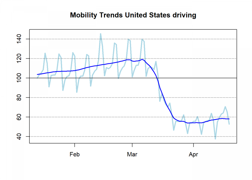
The drop is quite dramatic… by 60%! Even more dramatic, of course, is the situation in Italy:
mobi_trends(reg = "Italy")
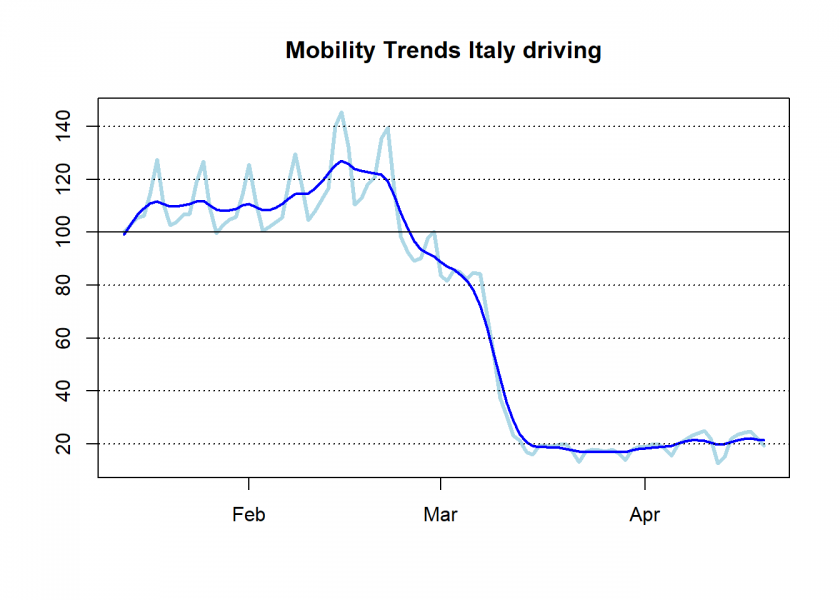
A drop by 80%! The same plot for Frankfurt:
mobi_trends(reg = "Frankfurt")
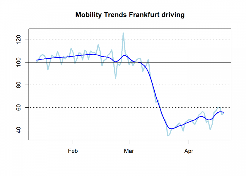
Obviously in Germany people are taking those measures less seriously lately, there seems to be a clear upward trend. This can also be seen in the German “walking” data:
mobi_trends(reg = "Germany", trans = "walking")
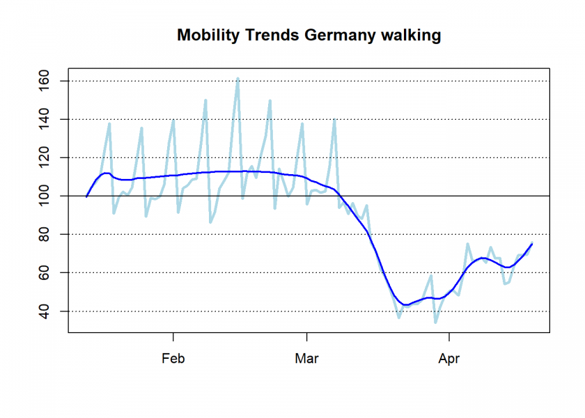
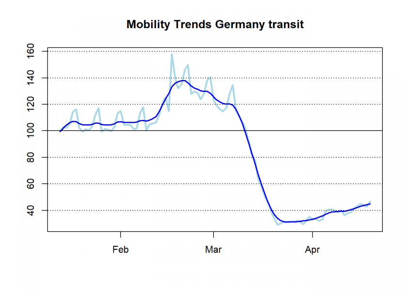
What is interesting is that before the lockdown “transit” mobility seems to have accelerated before plunging:
mobi_trends(reg = "Germany", trans = "transit")
You can also plot the raw numbers only, without an added smoother (option addsmooth = FALSE):
mobi_trends(reg = "London", trans = "walking", addsmooth = FALSE)
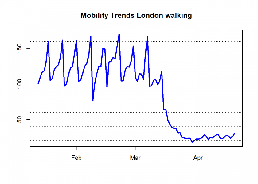
And as I said, you can conduct your own analyses on the formatted vector of the time series (option plot = FALSE)…
mobi_trends(reg = "London", trans = "walking", plot = FALSE)
## 2020-01-13 2020-01-14 2020-01-15 2020-01-16 2020-01-17 2020-01-18
##     100.00     108.89     116.84     118.82     132.18     160.29
## 2020-01-19 2020-01-20 2020-01-21 2020-01-22 2020-01-23 2020-01-24
##     105.12     108.02     120.52     124.81     127.01     137.38
## 2020-01-25 2020-01-26 2020-01-27 2020-01-28 2020-01-29 2020-01-30
##     162.41      97.16     100.01     113.27     122.75     124.96
## 2020-01-31 2020-02-01 2020-02-02 2020-02-03 2020-02-04 2020-02-05
##     144.13     161.17     103.93     105.67     115.03     125.42
## 2020-02-06 2020-02-07 2020-02-08 2020-02-09 2020-02-10 2020-02-11
##     128.43     140.65     167.80      76.79     100.51     115.26
## 2020-02-12 2020-02-13 2020-02-14 2020-02-15 2020-02-16 2020-02-17
##     125.35     124.69     150.77     149.35      96.03     131.20
## 2020-02-18 2020-02-19 2020-02-20 2020-02-21 2020-02-22 2020-02-23
##     131.72     137.59     136.05     153.95     170.22     104.41
## 2020-02-24 2020-02-25 2020-02-26 2020-02-27 2020-02-28 2020-02-29
##     104.32     119.88     125.12     123.88     133.76     153.92
## 2020-03-01 2020-03-02 2020-03-03 2020-03-04 2020-03-05 2020-03-06
##     109.26     103.64     114.68     114.25     106.50     142.09
## 2020-03-07 2020-03-08 2020-03-09 2020-03-10 2020-03-11 2020-03-12
##     167.10      96.86      97.50     105.54     106.91      98.87
## 2020-03-13 2020-03-14 2020-03-15 2020-03-16 2020-03-17 2020-03-18
##     104.19     117.44      64.28      64.53      48.95      43.31
## 2020-03-19 2020-03-20 2020-03-21 2020-03-22 2020-03-23 2020-03-24
##      38.76      37.49      37.36      30.76      31.25      24.63
## 2020-03-25 2020-03-26 2020-03-27 2020-03-28 2020-03-29 2020-03-30
##      24.09      22.89      23.40      23.40      17.83      19.72
## 2020-03-31 2020-04-01 2020-04-02 2020-04-03 2020-04-04 2020-04-05
##      22.29      22.19      22.76      24.34      28.49      26.06
## 2020-04-06 2020-04-07 2020-04-08 2020-04-09 2020-04-10 2020-04-11
##      21.63      24.64      23.87      26.13      28.59      28.58
## 2020-04-12 2020-04-13 2020-04-14 2020-04-15 2020-04-16 2020-04-17
##      22.86      22.80      25.66      27.44      26.40      23.27
## 2020-04-18 2020-04-19
##      26.36      30.40
…as we have only scratched the surface of the many possibilities here, there are many interesting analyses, like including the data in epidemiological models or simply calculate correlations with new infections/deaths: please share your findings in the comments below!
One thought on “COVID-19: Analyze Mobility Trends with R”