
Public-key cryptography is one of the foundations of our modern digital life. Normally it is quite hard to understand but with our literally colourful explanation it is a walk in the park. At the end we also give the nerd version, so read on!
One problem with cryptography is that you often would like to have a shared secret key to encrypt and decrypt messages (e.g. credit card information) but you of course cannot just send the secret key to the other party unencrypted – now you see the problem!
We want to find a method to generated a shared secret key by only sending publicly observable information. “Impossible”, you say? No, only ingenious!
Let me start by presenting a riddle to you: say, you want to have a box with some valuables delivered to a friend of yours but you don’t trust the carrier. You and your friend are allowed to use locks but you don’t have a lock for which you and your friend have a key. You can also send the box back and forth as often as you want. What to do? Think about it for a moment, I’ll wait…

…ok, here is a possible solution: You put a lock on the box, for which only you have the key. The box is delivered to your friend. Your friend puts on another lock, for which only he has the key and sends it back to you, now with two locks on. You remove your lock and send it back to him one last time, problem solved!
The method we are going to explain is designed in a very much the same spirit. It is called “Diffie–Hellman key exchange” and was one of the first so-called public-key protocols and is still widely used today.
The following explanation based on mixing colours is not new but here we not only do it illustratively but demonstrate it by actually mixing colours with R!
We will use the MixColor() function from the versatile DescTools package (on CRAN). First we write a small helper function for mixing the colours, plotting the result and returning the RGB (Red-Green-Blue) code of the new colour:
library(DescTools)

mix_col <- function(col1, col2 = col1, amount1 = 0.5, main = "") {
  mix_col <- MixColor(col1, col2, amount1)
  plot(0, type = 'n', xlim = c(0, 100), ylim = c(0, 100), axes = FALSE, xlab = "", ylab = "", main = main)
  rect(0, 0, 100, 100, col = mix_col)
  mix_col
}
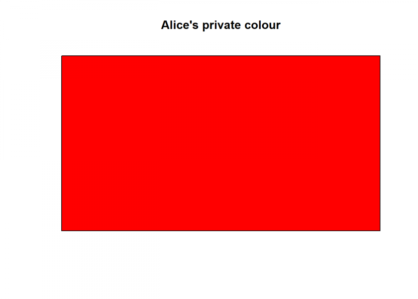
Both parties, traditionally called Alice and Bob, start out with their own private colour which they will keep secret:
Alices_private_col <- "red"
mix_col(Alices_private_col, main = "Alice's private colour")
## [1] "#FF0000FF"
Bobs_private_col <- "blue"
mix_col(Bobs_private_col, main = "Bob's private colour")
## [1] "#0000FFFF"

On top of that, we need a public colour:
public_col <- "green"
mix_col(public_col, main = "Public colour")
## [1] "#00FF00FF"

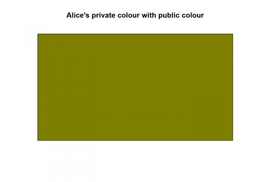
Now, the fun can begin! Alice takes her private colour (red), mixes it with the public colour (green) and sends the result publicly to Bob…
(Alice2Bob <- mix_col(Alices_private_col, public_col, main = "Alice's private colour with public colour"))
## [1] "#7F7F00FF"
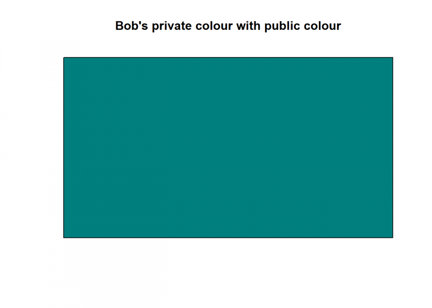
…and Bob takes his private colour (blue), mixes it with the public colour (green) and sends the result publicly to Alice:
(Bob2Alice <- mix_col(Bobs_private_col, public_col, main = "Bob's private colour with public colour"))
## [1] "#007F7FFF"
So far, so good. And now for the final step: Both take the colour the other party has sent them and mix it with their own private secret colour (in the ratio 2/3 to 1/3, so that all three colours share 1/3 of the total):
mix_col(Bob2Alice, Alices_private_col, amount = 2/3, main = "Shared secret colour")
## [1] "#545454FF"

mix_col(Alice2Bob, Bobs_private_col, amount = 2/3, main = "Shared secret colour")
## [1] "#545454FF"
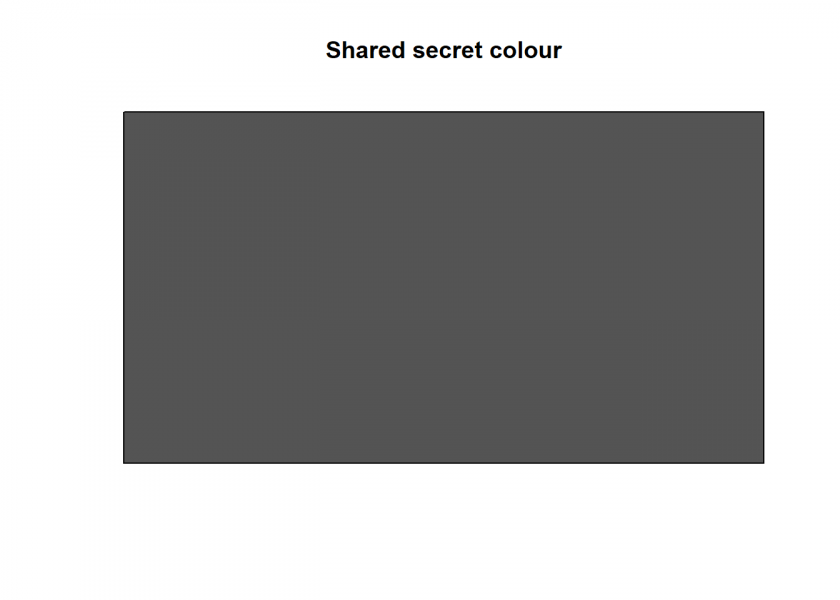
As can be seen, the result is the same secret – but now shared – colour. This method works because there is some asymmetry involved: It is easy to mix colours but very hard to undo that! Even if a hostile third party, traditionally called Eve, was listening in, she couldn’t make sense of the intercepted data.
Now that you understand the general principle, as promised, for the nerd version:
We need a mathematical equivalent of our colour mixing: a function that is simple to calculate in our direction but hard in the other. Those functions indeed exist and are called trapdoor functions.
You don’t have to look any further than dividing a simple exponentiation by some number and only keeping the remainder (which is the modulo function, or %% in R). Those numbers have to fulfil certain prerequisites like being prime and being very long random numbers but the principle is the same: simple to calculate in one direction but very hard in the other (in this case the reason is what is known under the name “discrete logarithm problem” but we won’t give any more details here).
When you have a look at the following fully documented toy example you will recognize the same principle at work as with the colours above:
Alices_private_no <- 15
Bobs_private_no <- 13
prime <- 17 # public prime
generator <- 3 # public generator

(Alice2Bob <- generator^Alices_private_no %% prime) # Alice selects private random number (15) and sends result  (6) publicly to Bob
## [1] 6

(Bob2Alice <- generator^Bobs_private_no %% prime)   # Bob   selects private random number (13) and sends result (12) publicly to Alice
## [1] 12

# shared secret key
Bob2Alice^Alices_private_no %% prime # Alice takes Bob's public result (12), raises it to her private random number (15) modulo the public prime number (17)
## [1] 10

Alice2Bob^Bobs_private_no %% prime   # Bob takes Alice's public result  (6), raises it to his private random number (13) modulo the public prime number (17)
## [1] 10
Fascinating, isn’t it? And now you can understand the principle behind this foundational technology!
Let me end this post with a well-kept secret about nerds:
