

Noseman is having a headache and as an old-school hypochondriac he goes to see his doctor. His doctor is quite worried and makes an appointment with a radiologist for Noseman to get a CT scan.
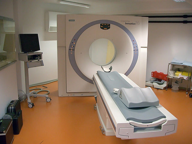
Because Noseman always wants to know how things work he asks the radiologist about the inner workings of a CT scanner.
The basic idea is that X-rays are fired from one side of the scanner to the other. Because different sorts of tissue (like bones, brain cells, cartilage, etc.) block different amounts of the X-rays the intensity measured on the other side varies accordingly.
The problem is of course that a single picture cannot give the full details of what is inside the body because it is a combination of different sorts of tissue in the way of the respective X-rays. The solution is to rotate the scanner and combine the different slices.
How, you ask? Good old linear algebra to the rescue!
We start with the initial position and fire X-rays with an intensity of 30 (just a number for illustrative purposes) through the body:
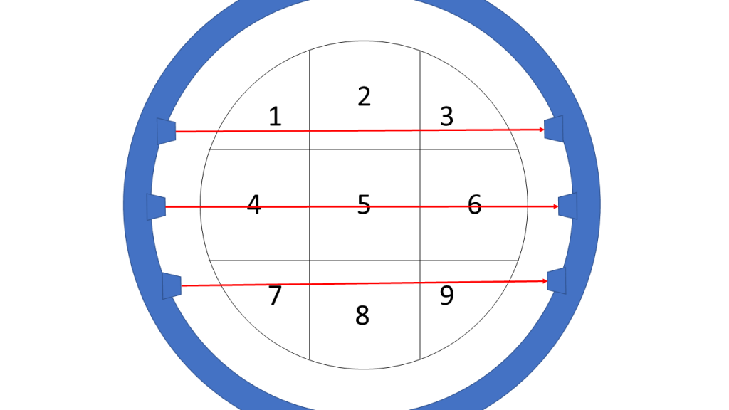
As can be seen in the picture the upper ray goes through areas 1, 2 and 3 and let’s say that the intensity value of 12 is measured on the other side of the scanner:
![\[30-x_1-x_2-x_3=12\]](https://blog.ephorie.de/wp-content/ql-cache/quicklatex.com-066468d5466dcbf8c9e97f7896906875_l3.png "Rendered by QuickLaTeX.com")
or
![\[x_1+x_2+x_3=18\]](https://blog.ephorie.de/wp-content/ql-cache/quicklatex.com-41d730ac56d073cd95221de26b6b2d43_l3.png "Rendered by QuickLaTeX.com")
The rest of the formula is found accordingly:
![\[\underbrace{ \begin{pmatrix} 1 & 1 & 1 & 0 & 0 & 0 & 0 & 0 & 0 \\ 0 & 0 & 0 & 1 & 1 & 1 & 0 & 0 & 0 \\ 0 & 0 & 0 & 0 & 0 & 0 & 1 & 1 & 1 \end{pmatrix} }_{\bold{A}_1} \underbrace{ \begin{pmatrix} x_1 \\ x_2 \\ x_3 \\ x_4 \\ x_5 \\ x_6 \\ x_7 \\ x_8 \\ x_9 \end{pmatrix} }_{\bold{x}} = \underbrace{ \begin{pmatrix} 18 \\ 21 \\ 18 \end{pmatrix} }_{\bold{b}_1}\]](https://blog.ephorie.de/wp-content/ql-cache/quicklatex.com-851b62bfdf021a0bee93b5448493147a_l3.png "Rendered by QuickLaTeX.com")
We then rotate the scanner for the first time…
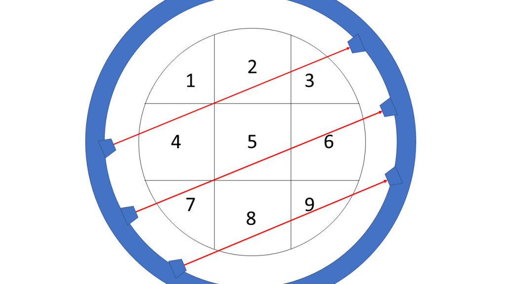
…which gives the following formula:
![\[\underbrace{ \begin{pmatrix} 0 & 1 & 1 & 1 & 0 & 0 & 0 & 0 & 0 \\ 0 & 0 & 0 & 0 & 1 & 1 & 1 & 0 & 0 \\ 0 & 0 & 0 & 0 & 0 & 0 & 0 & 1 & 1 \end{pmatrix} }_{\bold{A}_2} \underbrace{ \begin{pmatrix} x_1 \\ x_2 \\ x_3 \\ x_4 \\ x_5 \\ x_6 \\ x_7 \\ x_8 \\ x_9 \end{pmatrix} }_{\bold{x}} = \underbrace{ \begin{pmatrix} 18 \\ 21 \\ 9 \end{pmatrix} }_{\bold{b}_2}\]](https://blog.ephorie.de/wp-content/ql-cache/quicklatex.com-de165b533a8f803b666d71386b3611b9_l3.png "Rendered by QuickLaTeX.com")
And a second rotation…
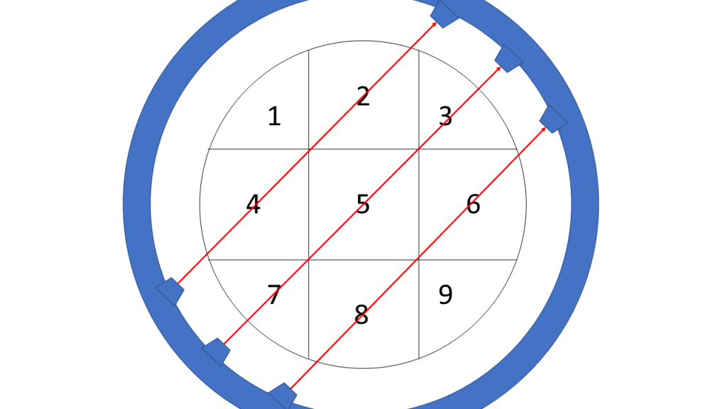
…yields the following formula:
![\[\underbrace{ \begin{pmatrix} 0 & 1 & 0 & 1 & 0 & 0 & 0 & 0 & 0 \\ 0 & 0 & 1 & 0 & 1 & 0 & 1 & 0 & 0 \\ 0 & 0 & 0 & 0 & 0 & 1 & 0 & 1 & 0 \end{pmatrix} }_{\bold{A}_3} \underbrace{ \begin{pmatrix} x_1 \\ x_2 \\ x_3 \\ x_4 \\ x_5 \\ x_6 \\ x_7 \\ x_8 \\ x_9 \end{pmatrix} }_{\bold{x}} = \underbrace{ \begin{pmatrix} 18 \\ 14 \\ 16 \end{pmatrix} }_{\bold{b}_3}\]](https://blog.ephorie.de/wp-content/ql-cache/quicklatex.com-5f587270a063ead84ef2366ef169b317_l3.png "Rendered by QuickLaTeX.com")
Now we are combining all three systems of equations:
![\[\begin{pmatrix} \bold{A}_1 \\ \bold{A}_2 \\ \bold{A}_3 \end{pmatrix} \bold{x} = \begin{pmatrix} \bold{b}_1 \\ \bold{b}_2 \\ \bold{b}_3 \end{pmatrix}\]](https://blog.ephorie.de/wp-content/ql-cache/quicklatex.com-cfaadd4a0fa0291fcd0e3adc0336e152_l3.png "Rendered by QuickLaTeX.com")
or written out in full:
![\[\underbrace{ \begin{pmatrix} 1 & 1 & 1 & 0 & 0 & 0 & 0 & 0 & 0 \\ 0 & 0 & 0 & 1 & 1 & 1 & 0 & 0 & 0 \\ 0 & 0 & 0 & 0 & 0 & 0 & 1 & 1 & 1 \\ 0 & 1 & 1 & 1 & 0 & 0 & 0 & 0 & 0 \\ 0 & 0 & 0 & 0 & 1 & 1 & 1 & 0 & 0 \\ 0 & 0 & 0 & 0 & 0 & 0 & 0 & 1 & 1 \\ 0 & 1 & 0 & 1 & 0 & 0 & 0 & 0 & 0 \\ 0 & 0 & 1 & 0 & 1 & 0 & 1 & 0 & 0 \\ 0 & 0 & 0 & 0 & 0 & 1 & 0 & 1 & 0 \end{pmatrix} }_{\bold{A}} \underbrace{ \begin{pmatrix} x_1 \\ x_2 \\ x_3 \\ x_4 \\ x_5 \\ x_6 \\ x_7 \\ x_8 \\ x_9 \end{pmatrix} }_{\bold{x}} = \underbrace{ \begin{pmatrix} 18 \\ 21 \\ 18 \\ 18 \\ 21 \\ 9 \\ 18 \\ 14 \\ 16 \end{pmatrix} }_{\bold{b}}\]](https://blog.ephorie.de/wp-content/ql-cache/quicklatex.com-3d36217792b9444190f0434bbd941507_l3.png "Rendered by QuickLaTeX.com")
Here is the data of the matrix  for you to download: ct-scan.txt).
We now have 9 equations with 9 unknown variables… which should easily be solvable by R, which can also depict the solution as a gray-scaled image… the actual CT-scan!
A <- read.csv("data/ct-scan.txt")
b <- c(18, 21, 18, 18, 21, 9, 18, 14, 16)
v <- solve(A, b)
matrix(v, ncol = 3, byrow = TRUE)
##      [,1] [,2] [,3]
## [1,]    9    9    0
## [2,]    9    5    7
## [3,]    9    9    0
image(matrix(v, ncol = 3), col = gray(4:0 / 4))
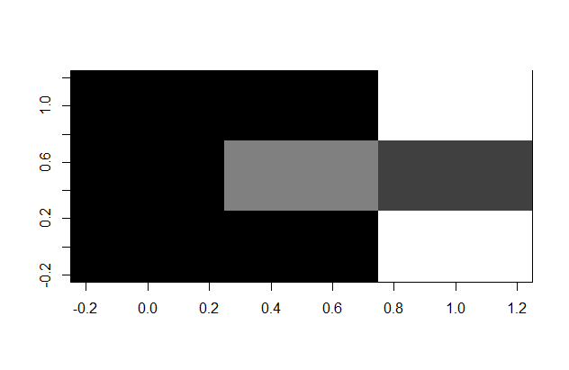
The radiologist looks at the picture… and has good news for Noseman: everything is how it should be! Noseman is relieved and his headache is much better now…
Real CT scans make use of the same basic principles (of course with a lot of additional engineering and maths magic 😉 )
Here are real images of CT scans of a human brain…
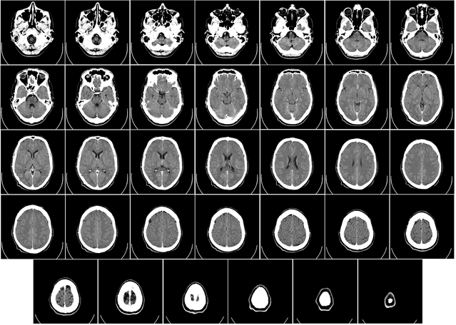
… which can be combined into a 3D-animation:
Isn’t it fascinating how a little bit of maths can save lives!
You can check out the brainspriteR package. I takes in slides from one plane to return a widget that displays inferred images from the other planes
https://github.com/oganm/brainspriteR
Thank you for the reference!
Nice, thank you! Matrix A seems to be A1 over A3 (instead of A2) over A3 (it is correct in ct-scan.txt).
Thank you for catching the mistake, Rolf! Corrected it.
Learnt something new today. Thank you.
You are very welcome!
We now have 9 equations with 9 unknown variables… which should easily be solvable by R
… but det(A) = 0. Then ¿?
Are there any scanners that tilt the plane of the xrays relative to the subject? Would that improve the resolution? Or would the additional complexity not be a (net) benefit?