

Principal Component Analysis (PCA) is a dimension-reduction method that can be used to reduce a large set of (often correlated) variables into a smaller set of (uncorrelated) variables, called principal components, which still contain most of the information.
PCA is a concept that is traditionally hard to grasp so instead of giving you the n’th mathematical derivation I will provide you with some intuition.
Basically, PCA is nothing else but a projection of some higher dimensional object into a lower dimension. What sounds complicated is really something we encounter every day: when we watch TV we see a 2D-projection of 3D-objects!
Please watch this instructive video:
So what we want is not only a projection but a projection which retains as much information as possible. A good strategy is to find the longest axis of the object and after that turn the object around this axis so that we again find the second longest axis.
Mathematically this can be done by calculating the so-called eigenvectors of the covariance matrix, after that we use just use the n eigenvectors with the biggest eigenvalues to project the object into n-dimensional space (in our example n = 2) – but as I said I won’t go into the mathematical details here (many good explanations can be found here on stackexchange).
To make matters concrete we will now recreate the example from the video above! The teapot data is from https://www.khanacademy.org/computer-programming/3d-teapot/971436783 – there you can also turn it around interactively.
Have a look at the following code:
library(scatterplot3d)
teapot <- read.csv("data/teapot.csv", header = FALSE)
dat <- matrix(unlist(teapot), ncol = 3, byrow = TRUE)
head(dat)
## [,1] [,2] [,3]
## [1,] 40.6 28.3 -1.1
## [2,] 40.1 30.4 -1.1
## [3,] 40.7 31.1 -1.1
## [4,] 42.0 30.4 -1.1
## [5,] 43.5 28.3 -1.1
## [6,] 37.5 28.3 14.5
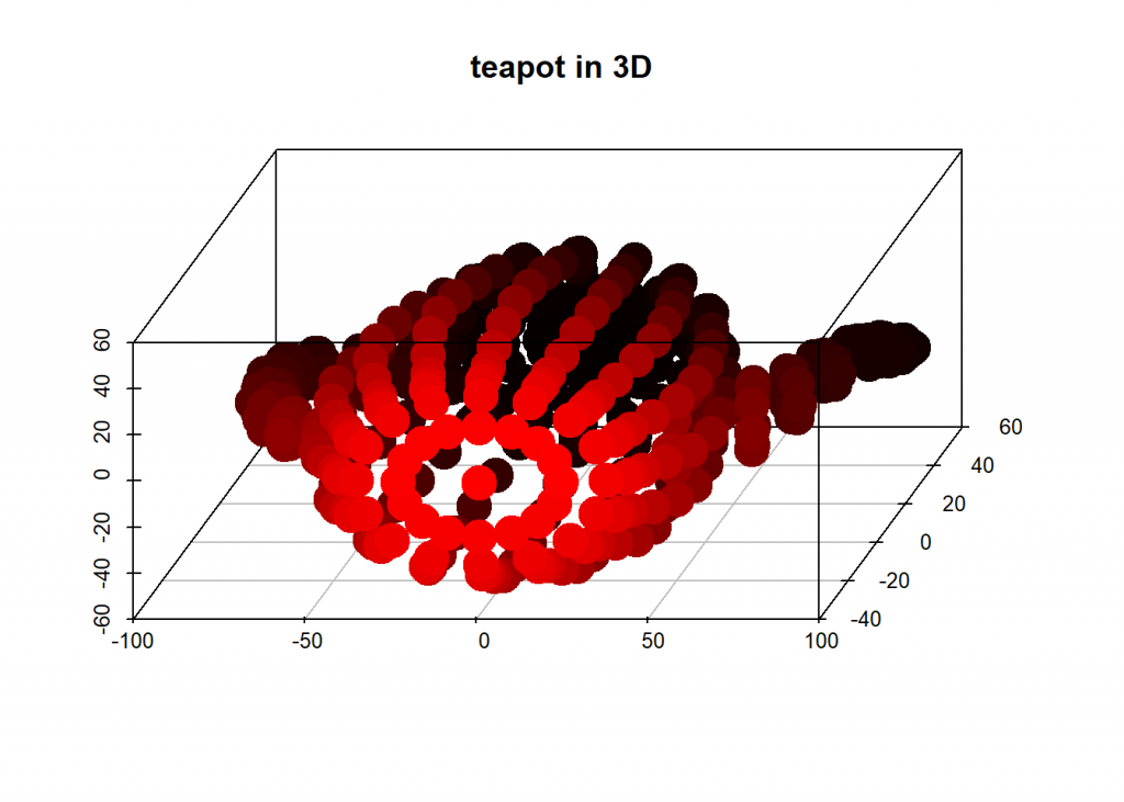
# teapot in 3D
scatterplot3d(dat[ , 1], dat[ , 2], dat[ , 3], highlight.3d = TRUE, angle = 75, pch = 19, lwd = 15, xlab = "", ylab = "", zlab = "", main = "teapot in 3D")
And now we project that teapot from 3D-space onto a 2D-plane while retaining as much information as possible by taking the two eigenvectors with biggest eigenvalues:
# PCA
(eigenval <- eigen(cov(dat))$values)
## [1] 2050.6935  747.5764  553.4070

eigenvec <- eigen(cov(dat))$vectors
# take only the two eigenvectors with biggest eigenvalues
PCA_2 <- dat %*% eigenvec[ , 1:2]
plot(PCA_2, ylim = c(50, -55), pch = 19, lwd = 35, col= "blue", xlab = "", ylab = "", main = "teapot in 2D")
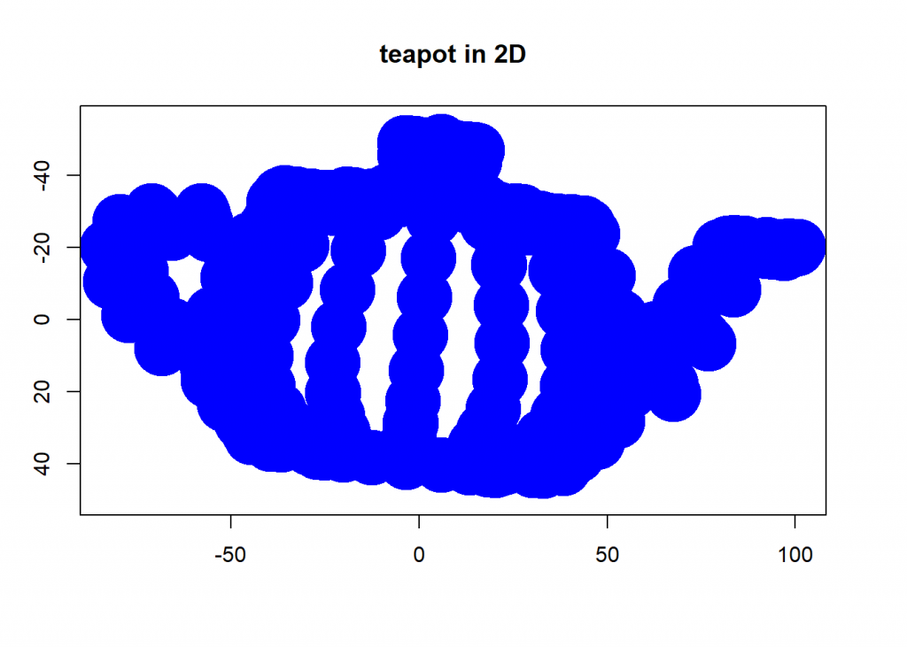
round(cumsum(eigenval)/sum(eigenval) * 100, 2) # cumulative percentage of retrieved information
## [1]  61.18  83.49 100.00
That was fun, wasn’t it!
In data science, you will often use PCA to condense large datasets into smaller datasets while retaining most of the information (which means retaining as much variance as possible in this case). PCA is like clustering an unsupervised learning method.
A total beginner’s question (to programming, not to statistics): How did you get the tea pot data into a csv file? Did you just copy/paste it? All of it or just the coordinates? I would like to replicate what you did.
And also: thank you for this informative post! Most people have (understandable) trouble wrapping their head around PCA, and this post is nice break-down of the basic principles.
Best, Ash
Thank you for your positive feedback, I really appreciate it.
It was basically just copy and paste (some of the other comments give details). The reason I don’t include the dataset for download is that I am not sure about copyright issues here.
I had the same problem – where to get the data. So I went to the cited URL, and copied the entire Processing program. Then in an ASCII editor (BBEdit in my case) I removed the clutter above and below the array, removed brackets, changed commas into tabs, and pasted into a spreadsheet. Then one can either directly import the spreadsheet with appropriate R libraries or export the spreadsheet as CSV.
The conversion to matrix was easier given that format:
dat = as.matrix(teapot).Thanks for a nice article helping my intuition here!
Best, Michael
I extracted the data the same way, then skipped converting it to a matrix because it was already in the format shown by
head(). Didn’t realize it would later need to be a matrix. 😉Code doesn’t work for me. Able to extract a csv from the link, and all wroks fine until this line:
returns error:
Found my problem. I needed to make dat a matrix.
It wasn’t a matrix because the data as read as a CSV was already in the format of your example, using the line:
resulted in a matrix that didn't work with the other parts of the example. It returns:
 head(dat)
     [,1] [,2] [,3]
[1,] 40.6 40.1 40.7
[2,] 42.0 43.5 37.5
[3,] 37.0 37.6 38.8
[4,] 40.2 29.1 28.7
[5,] 29.1 30.1 31.1
[6,] 16.5 16.2 16.5
So I skipped
because the data already looked like your example:
Not sure what's going on. Maybe your CSV file was shaped differently?
Glad that it works now!
Sometimes study through cases can be very beneficial for understanding.
An interesting case-study of PCA can be found here: https://iopscience.iop.org/article/10.1088/2632-2153/abd87c
This is the case where PCA was applied in conjunction with the K-means clustering to perform an advanced characterization of monolayer matter, where different physically distinct areas were identified.