

A few months ago I published a post on recursion: To understand Recursion you have to understand Recursion…. In this post we will see how to use recursion to fill free areas of an image with colour, the caveats of recursion and how to transform a recursive algorithm into a loop-based version using a queue – so read on…
The recursive version of the painting algorithm we want to examine here is very easy to understand, Wikipedia gives the pseudocode of the so called flood-fill algorithm:
Flood-fill (node, target-color, replacement-color):
- If target-color is equal to replacement-color, return.
- If the color of node is not equal to target-color, return.
- Set the color of node to replacement-color.
- Perform Flood-fill (one step to the south of node, target-color, replacement-color).
Perform Flood-fill (one step to the north of node, target-color, replacement-color).
Perform Flood-fill (one step to the west of node, target-color, replacement-color).
Perform Flood-fill (one step to the east of node, target-color, replacement-color). - Return.
The translation into R couldn’t be any easier:
floodfill <- function(row, col, tcol, rcol) {
  if (tcol == rcol) return()
  if (M[row, col] != tcol) return()
  M[row, col] <<- rcol
  floodfill(row - 1, col    , tcol, rcol) # south
  floodfill(row + 1, col    , tcol, rcol) # north
  floodfill(row    , col - 1, tcol, rcol) # west
  floodfill(row    , col + 1, tcol, rcol) # east
  return("filling completed")
}
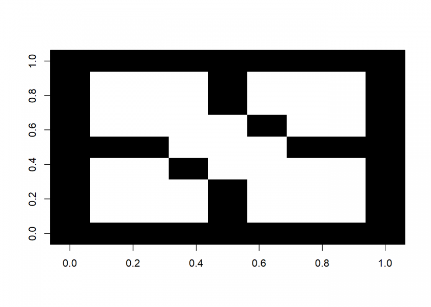
We take the image from Wikipedia as an example:
M <- matrix(c(1, 1, 1, 1, 1, 1, 1, 1, 1,
              1, 0, 0, 0, 1, 0, 0, 0, 1,
              1, 0, 0, 0, 1, 0, 0, 0, 1,
              1, 0, 0, 1, 0, 0, 0, 0, 1,
              1, 1, 1, 0, 0, 0, 1, 1, 1,
              1, 0, 0, 0, 0, 1, 0, 0, 1,
              1, 0, 0, 0, 1, 0, 0, 0, 1,
              1, 0, 0, 0, 1, 0, 0, 0, 1,
              1, 1, 1, 1, 1, 1, 1, 1, 1), 9, 9)
image(M, col = c(0, 1))
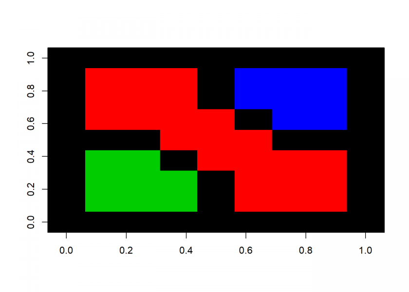
We now fill the three areas with three different colours and then plot the image again:
startrow <- 5; startcol <- 5
floodfill(startrow, startcol, 0, 2)
## [1] "filling completed"

startrow <- 3; startcol <- 3
floodfill(startrow, startcol, 0, 3)
## [1] "filling completed"

startrow <- 7; startcol <- 7
floodfill(startrow, startcol, 0, 4)
## [1] "filling completed"

image(M, col = 1:4)
This seems to work pretty well but the problem is that the more nested the algorithm becomes the bigger the stack has to be – which could lead to overflow errors. One comment on my original post on recursion read:
just keep in mind that recursion is useful in industrial work only if tail optimization is supported. otherwise your code will explode at some indeterminate time in the future. […]
One possibility is to increase the size of the stack with options(expressions = 10000) but even this may not be enough. Therefore we transform our recursive algorithm into a loop-based one and use a queue instead of a stack! The pseudocode from Wikipedia:
Flood-fill (node, target-color, replacement-color):
- If target-color is equal to replacement-color, return.
- If color of node is not equal to target-color, return.
- Set the color of node to replacement-color.
- Set Q to the empty queue.
- Add node to the end of Q.
- While Q is not empty:
- Set n equal to the first element of Q.
- Remove first element from Q.
- If the color of the node to the west of n is target-color,
set the color of that node to replacement-color and add that node to the end of Q. - If the color of the node to the east of n is target-color,
set the color of that node to replacement-color and add that node to the end of Q. - If the color of the node to the north of n is target-color,
set the color of that node to replacement-color and add that node to the end of Q. - If the color of the node to the south of n is target-color,
set the color of that node to replacement-color and add that node to the end of Q. - Continue looping until Q is exhausted.
- Return.
Because of the way the algorithm fills areas it is also called forest fire. Again, the translation into valid R code is straightforward:
floodfill <- function(row, col, tcol, rcol) {
  if (tcol == rcol) return()
  if (M[row, col] != tcol) return()
  Q <- matrix(c(row, col), 1, 2)
  while (dim(Q)[1] > 0) {
    n <- Q[1, , drop = FALSE]
    west  <- cbind(n[1]    , n[2] - 1)
    east  <- cbind(n[1]    , n[2] + 1)
    north <- cbind(n[1] + 1, n[2]    )
    south <- cbind(n[1] - 1, n[2]    )
    Q <- Q[-1, , drop = FALSE]
    if (M[n] == tcol) {
      M[n] <<- rcol
      if (M[west] == tcol)  Q <- rbind(Q, west)
      if (M[east] == tcol)  Q <- rbind(Q, east)
      if (M[north] == tcol) Q <- rbind(Q, north)
      if (M[south] == tcol) Q <- rbind(Q, south)
    }
  }
  return("filling completed")
}
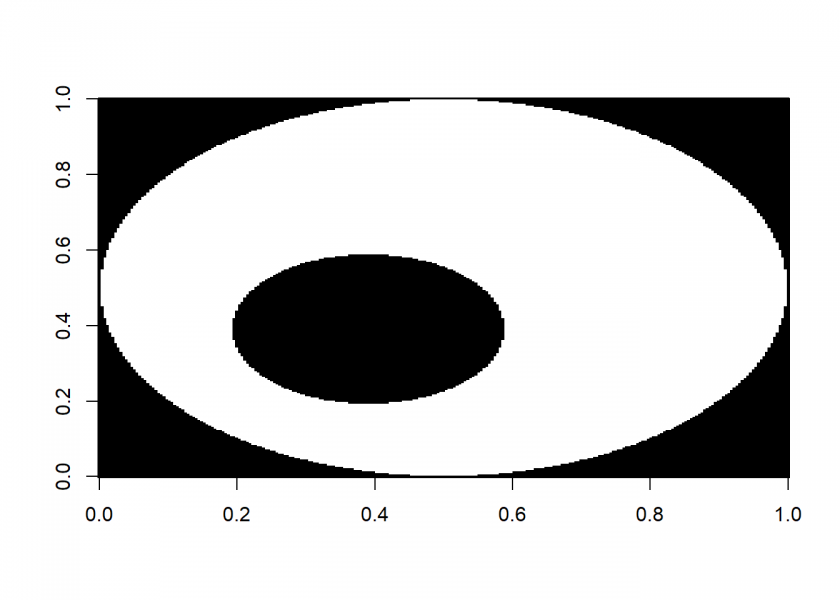
As an example we will use a much bigger picture (it can be downloaded from here: Unfilledcirc.png):
library(png)
img <- readPNG("data/Unfilledcirc.png")
M <- img[ , , 1]
M <- ifelse(M < 0.5, 0, 1)
M <- rbind(M, 0)
M <- cbind(M, 0)
image(M, col = c(1, 0))
And now for the filling:
startrow <- 100; startcol <- 100
floodfill(startrow, startcol, 0, 2)
## [1] "filling completed"

startrow <- 50; startcol <- 50
floodfill(startrow, startcol, 1, 3)
## [1] "filling completed"

image(M, col = c(1, 0, 2, 3))
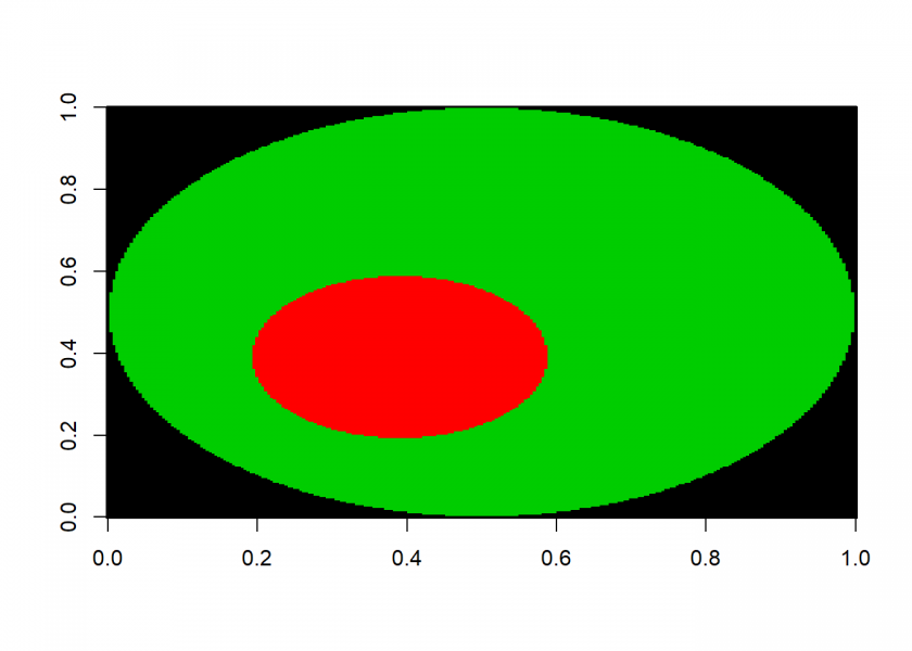
As you can see, with this version of the algorithm much bigger areas can be filled!
I also added both R implementations to the respective section of Rosetta Code: Bitmap/Flood fill.
Hi, the filling code is good, but use of “<<-" is frowned upon. In fact, CRAN will reject any submission using that.
How about simply passing the matrix M as an input argument and sending the modified M as an output? That has the added advantage of not "damaging" the source object if you got a parameter wrong.
I suppose that, in the recursion case, this might lead to a lot of unnecessary copies of M, so create a copy in some separate environment (not the .GlobalEnv) and access that environment.
I know, yet I used it for clarity and simplicity of the algorithm. Passing the matrix is of course superior in respect of side effects of the functions.
Carl, Could you perhaps provide a sketch of the code how to use a separate environment here? Thank you
Hi – I built some functions based on the instructions from “Mr. Flick” at the StackOverflow page
https://stackoverflow.com/questions/30416292/
It’s a bit (well, a LOT) confusing until you really get used to how to call and establish environments in R. But this code shows how to “hide” the value “count” in an environment that is not .GlobalEnv . The rest of your recursion code should work fine inside this nested environment.
.env<-(function() {
count <- 0
f <- function(x) {
count <<- count + 1
return( list(mean=mean(x), count=count))
}
return(environment())
})()
statfoo <- function(x){
list(.env$f(x),plus=2)
}
statbar <- function(x){
list(.env$f(x),minus=3)
}
Thank you, Carl… to be honest with you this looks a little bit intimidating (but that is obviously not your fault!).