Like most people, you will have used a search engine lately, like Google. But have you ever thought about how it manages to give you the most fitting results? How does it order the results so that the best are on top? Read on to find out!
The earliest search engines either had human-curated indices, like Yahoo! or used some simple heuristic like the more often the keyword you were looking for was mentioned on a page the better, like Altavista – which led to all kinds of crazy effects like certain keywords being repeated thousands of times on webpages to make them more “relevant”.
Now, most of those search engines are long gone because a new kid arrived on the block: Google! Google’s search engine results were much better than all of the competition and they became the dominant player in no time. How did they do that?
The big idea was in fact published by the two founders: Sergey Brin and Lawrence Page, it is called the pagerank algorithm (which is, of course, a pun because one of the authors was named Page too). The original paper was “S. Brin, L. Page: The Anatomy of a Large-Scale Hypertextual Web Search Engine”.
Let us start with another, related question: which properties are the best to own in Monopoly? Many would instinctively answer with the most expensive ones, i.e. Park Place and Boardwalk. But a second thought reveals that those might be the ones where you get the biggest rent if somebody lands on them but that the last part is the caveat… “IF” somebody lands on them! The best streets are actually the ones where players land on the most. Those happen to be the orange streets, St. James Place, Tennessee Avenue and New York Avenue and therefore they are the key to winning the game.
How do find those properties? For example by simulation: you just simulate thousands of dice rolls and see where the players land.
A similar idea holds true for finding the best web pages: you just start from a random position and simulate a surfer who visits different web pages by chance. For each surfing session, you tally the respective webpage where she ends up and after many runs, we get a percentage for each page. The higher this percentage is the more relevant the webpage!
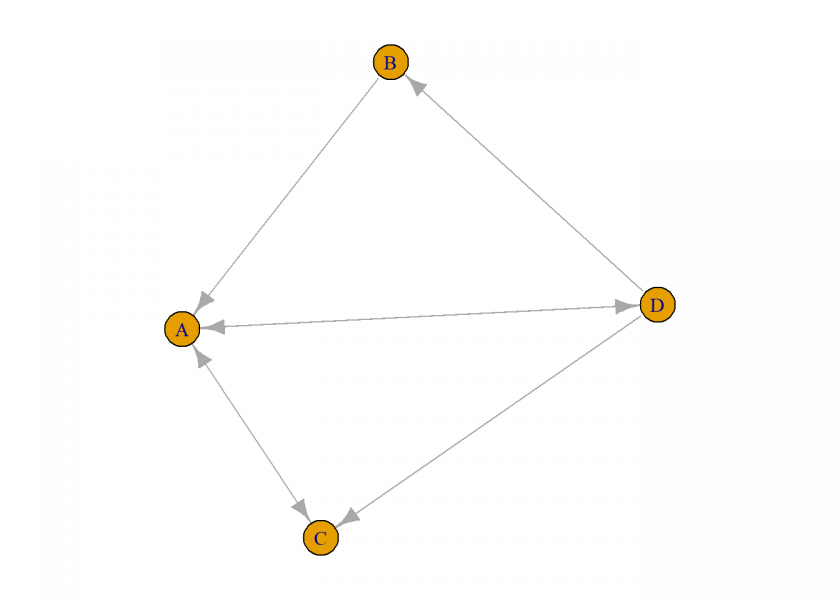
Let us do this with some R code. First we define a very small net and plot it (the actual example can be found in chapter 30 of the very good book “Chaotic Fishponds and Mirror Universes” by Richard Elwes):
library(igraph)
##
## Attaching package: 'igraph'
## The following objects are masked from 'package:stats':
##
##     decompose, spectrum
## The following object is masked from 'package:base':
##
##     union

# cols represent outgoing links, rows incoming links
# A links to C, D; B links to A; C links to A; D links to A,B,C
M <- matrix(c(0, 0, 1, 1,
              1, 0, 0, 0,
              1, 0, 0, 0,
              1, 1, 1, 0), nrow = 4)
colnames(M) <- rownames(M) <- c("A", "B", "C", "D")
M
##   A B C D
## A 0 1 1 1
## B 0 0 0 1
## C 1 0 0 1
## D 1 0 0 0

g <- graph_from_adjacency_matrix(t(M)) # careful with how the adjacency matrix is defined -> transpose of matrix

oldpar <- par(mar = c(1, 1, 1, 1))
plot(g)
par(oldpar)

Now, we are running the actual simulation. We define two helper functions for that, next_page for getting a random but possible next page given the page our surfer is on at the moment and last_page which gives the final page after N clicks:
next_page <- function(page, graph) {
  l <- sample(rownames(graph)[as.logical(graph[ , as.logical(page)])], 1)
  as.numeric(rownames(graph) == l)
}

last_page <- function(page, graph, N = 100) {
  for (i in seq(N)) {
    page <- next_page(page, graph)
  }
  page
}

current_page <- c(1, 0, 0, 0) # random surfer starting from A
random_surfer <- replicate(2e4, last_page(current_page, M, 50))
round(rowSums(random_surfer) / sum(random_surfer), 2)
## [1] 0.43 0.07 0.28 0.22
So we see that page A is the most relevant one because our surfer ends up being there in more than 40% of all sessions, after that come the pages C, D and B. When you look at the net that makes sense, since all pages refer to A whereas B gets only one link, so it doesn’t seem to be that relevant.
As you have seen the simulation even for this small net took quite long so we need some clever mathematics to speed up the process. One idea is to transform our matrix which represents the network into a matrix that gives the probabilities of landing on the next pages and then multiply the probability matrix with the current position (and thereby transform the probabilities). Let us do this for the first step:
M_prob <- prop.table(M, 2) # create probability matrix
M_prob
##     A B C         D
## A 0.0 1 1 0.3333333
## B 0.0 0 0 0.3333333
## C 0.5 0 0 0.3333333
## D 0.5 0 0 0.0000000

M_prob %*% current_page
##   [,1]
## A  0.0
## B  0.0
## C  0.5
## D  0.5
The result says that there is a fifty-fifty chance of landing on C or D. When you look at the graph you see that this is correct since there are two links, one to C and one to D! For the next step you would have to multiply the matrix with the result again, or first multiply the matrix with itself before multiplying with the current position, which gives:
![]()
If we want to do this a hundred times we just have to raise this probability matrix to the one-hundredth power:
![]()
We use the %^% operator in the expm package (on CRAN) for that:
library(expm)
## Loading required package: Matrix
##
## Attaching package: 'expm'
## The following object is masked from 'package:Matrix':
##
##     expm

r <- M_prob %^% 100 %*% current_page
r
##         [,1]
## A 0.42857143
## B 0.07142857
## C 0.28571429
## D 0.21428571
Again, we get the same result! You might ask: why ![]() ? The answer is that this is in most cases enough to get a stable result so that any further multiplication still results in the same result:
? The answer is that this is in most cases enough to get a stable result so that any further multiplication still results in the same result:
![]()
The last equations open up still another possibility: we are obviously looking for a vector ![]() which goes unaffected when multiplied by the matrix
which goes unaffected when multiplied by the matrix ![]() . There is a mathematical name for that kind of behaviour: eigenvector! As you might have guessed the name is an import from the German language where it means something like “own vector”.
. There is a mathematical name for that kind of behaviour: eigenvector! As you might have guessed the name is an import from the German language where it means something like “own vector”.
This hints at the problem we were solving all along (without consciously realizing perhaps): a page is the more relevant the more relevant a page is that links to it… now we have to know the importance of that page but that page two is the more relevant… and so on and so forth, we are going in circles here. The same is true when you look at the equation above: you define ![]() in terms of
in terms of ![]() –
– ![]() is the eigenvector of matrix
is the eigenvector of matrix ![]() !
!
There are very fast and powerful methods to find the eigenvectors of a matrix, and the corresponding eigen function is even a function in base R:
lr <- Re(eigen(M_prob)$vectors[ , 1]) # real parts of biggest eigenvector
lr / sum(lr) # normalization
## [1] 0.42857143 0.07142857 0.28571429 0.21428571
Again, the same result! You can now understand the title of this post and titles of other articles about the Pagerank algorithm and Google like “The $25,000,000,000 eigenvector”.
Yet, a word of warning is in order: there are cases where the probability matrix is not diagonalizable (we won’t get into the mathematical details here), which means that the eigenvector method won’t give sensible results. To check this the following code must evaluate to TRUE:
ev <- eigen(M_prob)$values
length(unique(ev)) == length(ev)
## [1] TRUE
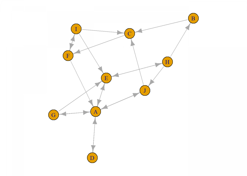
We now repeat the last two methods for a bigger network:
set.seed(1415)
n <- 10
g <- sample_gnp(n, p = 1/4, directed = TRUE) # create random graph
g <- set_vertex_attr(g, "name", value = LETTERS[1:n])
oldpar <- par(mar = c(1, 1, 1, 1))
plot(g)
par(oldpar)

M <- t(as_adjacency_matrix(g, sparse = FALSE))
M_prob <- prop.table(M, 2) # create probability matrix
M_prob
##      A B C D   E   F   G         H         I   J
## A 0.00 0 0 1 0.5 0.5 0.5 0.0000000 0.0000000 0.5
## B 0.00 0 0 0 0.0 0.0 0.0 0.3333333 0.0000000 0.0
## C 0.00 1 0 0 0.0 0.0 0.0 0.0000000 0.3333333 0.5
## D 0.25 0 0 0 0.0 0.0 0.0 0.0000000 0.0000000 0.0
## E 0.25 0 0 0 0.0 0.0 0.5 0.3333333 0.3333333 0.0
## F 0.00 0 1 0 0.0 0.0 0.0 0.0000000 0.3333333 0.0
## G 0.25 0 0 0 0.0 0.0 0.0 0.0000000 0.0000000 0.0
## H 0.00 0 0 0 0.5 0.0 0.0 0.0000000 0.0000000 0.0
## I 0.00 0 0 0 0.0 0.5 0.0 0.0000000 0.0000000 0.0
## J 0.25 0 0 0 0.0 0.0 0.0 0.3333333 0.0000000 0.0

current_page <- c(1, rep(0, n-1))
r <- M_prob %^% 100 %*% current_page
r
##         [,1]
## A 0.27663574
## B 0.02429905
## C 0.08878509
## D 0.06915881
## E 0.14579434
## F 0.10654199
## G 0.06915881
## H 0.07289723
## I 0.05327107
## J 0.09345787

lr <- Re(eigen(M_prob)$vectors[ , 1])
lr / sum(lr) # normalization of the real parts
##  [1] 0.27663551 0.02429907 0.08878505 0.06915888 0.14579439 0.10654206
##  [7] 0.06915888 0.07289720 0.05327103 0.09345794
We can now order the pages according to their importance – like the first 10 results of a google search:
search <- data.frame(Page = LETTERS[1:n], Rank = r)
search[order(search$Rank, decreasing = TRUE), ]
##   Page       Rank
## A    A 0.27663574
## E    E 0.14579434
## F    F 0.10654199
## J    J 0.09345787
## C    C 0.08878509
## H    H 0.07289723
## D    D 0.06915881
## G    G 0.06915881
## I    I 0.05327107
## B    B 0.02429905
Looking at the net, does the resulting order make sense to you?
Congratulations, you now understand the big idea behind one of the greatest revolutions in information technology!
Addendum: Extending PageRank to Financial Networks
The principles of Google’s PageRank algorithm also have significant applications in finance, specifically in analyzing interbank lending networks. Here, banks are nodes and loans are links. Understanding these connections helps assess systemic risks and manage financial stability.
In the financial sector, the failure of one bank can trigger a chain reaction of defaults. Thus, identifying which banks are critical for the overall system’s health is a key task for regulators. Using PageRank, they can determine which banks, termed as “Systemically Important Financial Institutions” (SIFIs), are most crucial. These banks are interconnected with other significant banks, much like important web pages are linked by other relevant sites. So, it is not “too big to fail” but “too interconnected to fail”!
This approach is employed by institutions such as the European Central Bank to monitor and support banks that are vital to averting financial crises. It demonstrates how mathematical models like PageRank can be adapted from the internet to finance, offering insights that help in targeted and effective regulatory interventions.

Very good. Thank you.
You are very welcome!