
 Networks are everywhere: traffic infrastructure and the internet come to mind, but networks are also in nature: food chains, protein-interaction networks, genetic interaction networks and of course neural networks which are being modelled by Artificial Neural Networks.
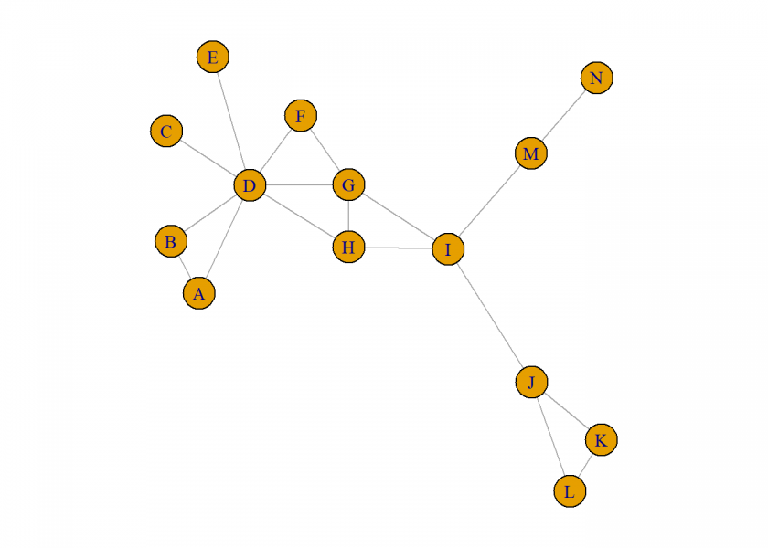
In this post, we will create a small network (also called graph mathematically) and ask some question about which is the “most important” node (also called vertex, pl. vertices). If you want to understand important concepts of network centrality and how to calculate those in R, read on!
This post is based on a LinkedIn post by renowned data scientist Dr. Keith McNulty. Let us (re-)create the small example network from there by first defining the adjacency matrix and after that plotting it with the igraph package (on CRAN). We have used this package already in another post on networks: Google’s Eigenvector… or: How a Random Surfer Finds the Most Relevant Webpages.
library(igraph)
## Warning: package 'igraph' was built under R version 4.0.2
##
## Attaching package: 'igraph'
## The following objects are masked from 'package:stats':
##
##     decompose, spectrum
## The following object is masked from 'package:base':
##
##     union

# define simple network
#             A, B, C, D, E, F, G, H, I, J, K, L, M, N
A <- matrix(c(0, 1, 0, 1, 0, 0, 0, 0, 0, 0, 0, 0, 0, 0, # A
              1, 0, 0, 1, 0, 0, 0, 0, 0, 0, 0, 0, 0, 0, # B
              0, 0, 0, 1, 0, 0, 0, 0, 0, 0, 0, 0, 0, 0, # C
              1, 1, 1, 0, 1, 1, 1, 1, 0, 0, 0, 0, 0, 0, # D
              0, 0, 0, 1, 0, 0, 0, 0, 0, 0, 0, 0, 0, 0, # E
              0, 0, 0, 1, 0, 0, 1, 0, 0, 0, 0, 0, 0, 0, # F
              0, 0, 0, 1, 0, 1, 0, 1, 1, 0, 0, 0, 0, 0, # G
              0, 0, 0, 1, 0, 0, 1, 0, 1, 0, 0, 0, 0, 0, # H
              0, 0, 0, 0, 0, 0, 1, 1, 0, 1, 0, 0, 1, 0, # I
              0, 0, 0, 0, 0, 0, 0, 0, 1, 0, 1, 1, 0, 0, # J
              0, 0, 0, 0, 0, 0, 0, 0, 0, 1, 0, 1, 0, 0, # K
              0, 0, 0, 0, 0, 0, 0, 0, 0, 1, 1, 0, 0, 0, # L
              0, 0, 0, 0, 0, 0, 0, 0, 1, 0, 0, 0, 0, 1, # M
              0, 0, 0, 0, 0, 0, 0, 0, 0, 0, 0, 0, 1, 0  # N
              ), nrow = 14)
colnames(A) <- rownames(A) <- LETTERS[1:ncol(A)]

A # adjacency matrix
##   A B C D E F G H I J K L M N
## A 0 1 0 1 0 0 0 0 0 0 0 0 0 0
## B 1 0 0 1 0 0 0 0 0 0 0 0 0 0
## C 0 0 0 1 0 0 0 0 0 0 0 0 0 0
## D 1 1 1 0 1 1 1 1 0 0 0 0 0 0
## E 0 0 0 1 0 0 0 0 0 0 0 0 0 0
## F 0 0 0 1 0 0 1 0 0 0 0 0 0 0
## G 0 0 0 1 0 1 0 1 1 0 0 0 0 0
## H 0 0 0 1 0 0 1 0 1 0 0 0 0 0
## I 0 0 0 0 0 0 1 1 0 1 0 0 1 0
## J 0 0 0 0 0 0 0 0 1 0 1 1 0 0
## K 0 0 0 0 0 0 0 0 0 1 0 1 0 0
## L 0 0 0 0 0 0 0 0 0 1 1 0 0 0
## M 0 0 0 0 0 0 0 0 1 0 0 0 0 1
## N 0 0 0 0 0 0 0 0 0 0 0 0 1 0

g <- graph_from_adjacency_matrix(A, mode = "undirected")
set.seed(258)
oldpar <- par(mar = c(1, 1, 1, 1))
plot(g)
par(oldpar)
McNulty writes in his post:
I love to use this example when I teach about network analysis. I ask the group: who is the most important person in this network?
Now, what does “most important” person mean? It of course depends on the definition and this is where network centrality measures come into play. We will have a look at three of those (there are many more out there…).
Degree centrality
McNulty explains:
Degree centrality tells you the most connected person: it is simply the number of nodes connected to each node, and it’s easy to see that D has the highest (7).
This is often the only metric given to identify “influencers”: how many followers do they have?
Degree centrality is easy to calculate in R (first “by hand”, after that with the igraph package):
rowSums(A)
## A B C D E F G H I J K L M N
## 2 2 1 7 1 2 4 3 4 3 2 2 2 1

degree(g)
## A B C D E F G H I J K L M N
## 2 2 1 7 1 2 4 3 4 3 2 2 2 1
Closeness centrality
McNulty explains:
Closeness centrality tells you who can propagate information quickest: you sum the path lengths from your node to each other node and then inverse it. G has four paths of length 1, 6 of length 2 and 3 of length 3. Which gives it a closeness centrality of 1/25. With the other main candidates I is 1/26, H is 1/26 and D is 1/27.
One application that comes to mind is identifying so-called superspreaders of infectious diseases, like COVID-19.
This is a little bit more involved, the simplest approach is to first convert the adjacency matrix to a distance matrix which measures the distances of the shortest paths from and to each node (I won’t go into the details, some pointers are given in the comments of the code):
# exponentiate the n x n adjacency matrix to the n'th power in the min-plus algebra. This is, instead of adding taking the minimum and instead of multiplying taking the sum.
# more details: https://en.wikipedia.org/wiki/Distance_matrix#Non-metric_distance_matrices

# distance product
"%C%" <- function(A, B) {
  n <- nrow(A)
  A[A == 0] <- Inf
  diag(A) <- 0
  B[B == 0] <- Inf
  diag(B) <- 0
  C <- matrix(0, nrow = n, ncol = n)
  for (i in 1:n) {
    for (j in 1:n) {
      tmp <- vector("integer", )
      for (k in 1:n) {
        tmp[k] <- A[i, k] + B[k, j]
      }
      C[i, j] <- min(tmp)
    }
  }
  colnames(C) <- rownames(C) <- rownames(A)
  C
}

# calculate distance matrix
DM <- function(A) {
  D <- A
  for (n in 1:nrow(A)) {
    D <- D %C% D
  }
  D
}

D <- DM(A) # distance matrix
D
##   A B C D E F G H I J K L M N
## A 0 1 2 1 2 2 2 2 3 4 5 5 4 5
## B 1 0 2 1 2 2 2 2 3 4 5 5 4 5
## C 2 2 0 1 2 2 2 2 3 4 5 5 4 5
## D 1 1 1 0 1 1 1 1 2 3 4 4 3 4
## E 2 2 2 1 0 2 2 2 3 4 5 5 4 5
## F 2 2 2 1 2 0 1 2 2 3 4 4 3 4
## G 2 2 2 1 2 1 0 1 1 2 3 3 2 3
## H 2 2 2 1 2 2 1 0 1 2 3 3 2 3
## I 3 3 3 2 3 2 1 1 0 1 2 2 1 2
## J 4 4 4 3 4 3 2 2 1 0 1 1 2 3
## K 5 5 5 4 5 4 3 3 2 1 0 1 3 4
## L 5 5 5 4 5 4 3 3 2 1 1 0 3 4
## M 4 4 4 3 4 3 2 2 1 2 3 3 0 1
## N 5 5 5 4 5 4 3 3 2 3 4 4 1 0

1 / rowSums(D)
##          A          B          C          D          E          F          G
## 0.02631579 0.02631579 0.02564103 0.03703704 0.02564103 0.03125000 0.04000000
##          H          I          J          K          L          M          N
## 0.03846154 0.03846154 0.02941176 0.02222222 0.02222222 0.02777778 0.02083333

closeness(g)
##          A          B          C          D          E          F          G
## 0.02631579 0.02631579 0.02564103 0.03703704 0.02564103 0.03125000 0.04000000
##          H          I          J          K          L          M          N
## 0.03846154 0.03846154 0.02941176 0.02222222 0.02222222 0.02777778 0.02083333
Betweenness centrality
McNulty explains:
Betweenness centrality tells you who is most important in maintaining connection throughout the network: it is the number of times your node is on the shortest path between any other pair of nodes. I uniquely connects all nodes on the left with all nodes on the right, which means it connects at 8×5 = 40 pairs, plus any node in the top right with the bottom right, a further 6 pairs, so 46 in total. If you follow a similar process for D, H and G you’ll see that they don’t come close to this.
For example in protein-interaction networks, betweenness centrality can be used to find important proteins in signalling pathways which can form targets for drug discovery.
The actual algorithm to calculate betweenness centrality is much too involved to show here (if you have a simple to understand algorithm please let me know on StackOverflow or in the comments), so we will just make use of the igraph package to calculate it:
betweenness(g)
##    A    B    C    D    E    F    G    H    I    J    K    L    M    N
##  0.0  0.0  0.0 41.5  0.0  0.0 21.5 15.0 46.0 22.0  0.0  0.0 12.0  0.0
As we have seen, there is more than one definition of “most important”. It will depend on the context (and the available information) which one to choose.
Please let me know your thoughts in the comments and please share further possible applications with us.
We’re taking our summer break! Look forward to the next post on October 6, 2020… and stay healthy!
Very nice article.
Any social media link to follow/subscribe to posts?
Thank you, highly appreciated! You can find me here:
LinkedIn: https://de.linkedin.com/in/vonjd (please click “Follow” if we don’t know each other or haven’t interacted in any way, if you want to connect please add at least a note)
Twitter: vonjd @ephorie
Very interesting. I liked the post. I’m still new to this graph thing, but I would like to know what are the units of centrality measures? I understand that in your example these are arbitrary units, but how does this relate to the length of the edges, for instance?
Cheers,
Mauro
Thank you, Mauro.
The units depend on the definition and context of the respective measure, e.g. with degree centrality it is the number of nodes (e.g. the number of followers in the context of social media).
There are generalizations for weighted graphs, see e.g.: Node centrality in weighted networks: Generalizing degree and shortest paths.