

When you ask successful people for their advice on how to become successful you will often hear that you have to take risks, often huge risks.
In this post we will examine whether this is good advice with a simple multi-agent simulation, so read on!
The following quotes from Dan Pierce are only two examples of a wealth of similar advice:
I am not where I am because of luck. I am where I am because I took risks others weren’t willing to take. The world rewards the risk-takers. It always has. It always will.
and
Only those willing to truly risk everything will gain everything. No person ever rose to greatness without the willingness to lose it all.
In a former post, we already found out with the help of a computer simulation that the distribution of wealth in the real world is indistinguishable from a distribution that is solely based on luck (see: The Rich didn’t earn their Wealth, they just got Lucky), here we will go one step further and actually simulate two types of agents: risk-takers (Risktakers) and “normal” people (Normals).
In every transaction Risktakers always risk all they possess, only limited by what their counterpart is willing to risk. Normals only risk up to 10% of their wealth. For the sake of comparability, we assume that all agents are equally skilled, so their only differentiator is their respective willingness to take risks.
It also means that when nobody is any better than the other the result of every transaction is purely based on luck. In this way, we make sure to isolate the sole effect of risk-taking and don’t mix it up with other qualities.
We are starting with 10,000 agents with an initial wealth of 1,000 units each. 10% of those are Risktakers, the rest are Normals. They conduct 2 million transactions with each other (NB: the simulation will take some time to run!):
w <- 1000 # initial wealth
s <- 10000 # population size
N <- 2e6 # no of transactions

set.seed(1234)
P <- rep(w, s) # creating population
p_rt <- 0.1 # proportion risk takers
max_ra <- 1 # risk appetite of Risktakers, 1 = 100%
n_ra <- 0.1 # risk appetite of Normals
names(P) <- c(rep(max_ra, p_rt*s), rep(n_ra, (1-p_rt)*s)) # risk appetite


for (i in seq_len(N) {
  who <- sample(s, size = 2) # draw two agents for the transaction
  profit <- min(as.numeric(names(P[who[1]]))*P[who[1]], as.numeric(names(P[who[2]]))*P[who[2]])
  luck <- sample(c(1, 2)) # who comes in first wins the profit!
  P[who[luck[1]]] <- P[who[luck[1]]] + profit
  P[who[luck[2]]] <- P[who[luck[2]]] - profit
}

Risktakers <- P[1:(p_rt*s)]
Normals <- P[(p_rt*s+1):s]

summary(Risktakers)
##    Min. 1st Qu.  Median    Mean 3rd Qu.    Max.
##     0.0     0.0     0.0   959.1     0.0 62525.8

summary(Normals)
##      Min.   1st Qu.    Median      Mean   3rd Qu.      Max.
##     0.181    92.055   385.436  1004.545  1322.948 12550.787
Just looking at the max values it seems that risk-taking really pays off bigly! The richest guy in town, with over 60,000 units, is a Risktaker! He increased his wealth more than sixtyfold! The richest Normal only has a comparable meager twelve thousand units. Risktaker beats Normal more than fivefold!
But wait, there is more…
Looking at the quartiles reveals that within the respective groups, wealth is distributed extremely unequally. Because the simulation is a zero-sum game the means are at about the initial wealth (Risktakers are a little bit lower but this is due to chance and can vary in different runs).
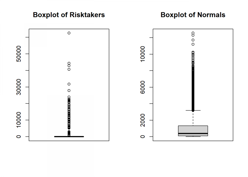
Yet all of the displayed quartiles of the Risktakers are zero! Let us visualize this with some boxplots and histograms:
par_bkp <- par(mfrow = c(1, 2)) # plot two plots side-by-side
boxplot(Risktakers, main = "Boxplot of Risktakers")
boxplot(Normals, main = "Boxplot of Normals")
hist(Risktakers, col = "red")
hist(Normals, col = "red")
par(par_bkp)
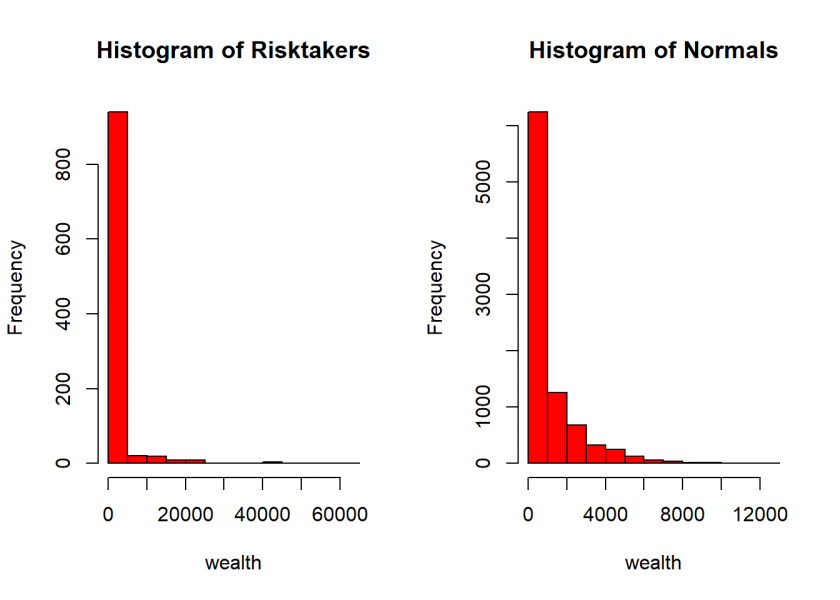
As you can again see, the distribution of wealth is extremely skewed a.k.a. fat-tailed in both cases but dramatically more so within the Risktaker’s group (as one can see in the boxplot, the outliers literally crush the rest of the rest of the distribution)! Where does this leave us for the overall population? Well, let’s have a look at the wealthiest one hundred agents:
head(sort(P, decreasing = TRUE), 100)
##         1         1         1         1         1         1         1         1
## 62525.762 44291.214 42917.925 40677.429 31761.799 27872.380 23929.614 22753.382
##         1         1         1         1         1         1         1         1
## 22458.062 22030.760 21756.148 21544.639 20970.771 20688.107 19473.726 19060.899
##         1         1         1         1         1         1         1         1
## 18342.086 18235.872 17411.690 16657.627 16277.219 16040.849 15266.584 14974.140
##         1         1         1         1         1         1         1         1
## 14156.247 14074.310 13847.214 13801.259 13729.240 13269.559 12951.397 12678.964
##       0.1       0.1         1         1       0.1         1       0.1         1
## 12550.787 12292.314 12002.368 11880.507 11715.641 11353.729 11193.644 10565.727
##         1         1         1         1         1       0.1       0.1       0.1
## 10532.670 10432.977 10385.944 10325.536 10266.249 10234.399 10178.293  9997.527
##       0.1         1       0.1       0.1       0.1       0.1         1       0.1
##  9995.841  9949.251  9834.962  9631.738  9439.200  9421.867  9359.496  9228.859
##       0.1         1       0.1       0.1       0.1       0.1         1       0.1
##  9224.529  9100.988  9029.623  9010.158  8910.210  8834.733  8711.897  8593.258
##       0.1       0.1       0.1       0.1       0.1       0.1       0.1         1
##  8543.662  8499.000  8404.759  8381.012  8373.831  8224.851  8190.105  8128.396
##       0.1       0.1       0.1       0.1       0.1       0.1       0.1       0.1
##  8107.256  8082.884  8080.619  8034.135  8033.168  7969.405  7955.725  7853.086
##       0.1       0.1       0.1       0.1       0.1       0.1       0.1       0.1
##  7809.438  7808.043  7778.937  7778.018  7759.078  7717.847  7681.713  7681.675
##       0.1         1       0.1       0.1       0.1       0.1       0.1       0.1
##  7671.718  7656.077  7654.444  7633.274  7617.269  7606.583  7562.145  7532.091
##       0.1       0.1       0.1       0.1
##  7518.953  7498.719  7483.523  7450.844
The top 30 comprises exclusively risk-takers (labeled 1 for 100% risk appetite) but…
tail(sort(P, decreasing = TRUE), 100)
## 1 1 1 1 1 1 1 1 1 1 1 1 1 1 1 1 1 1 1 1 1 1 1 1 1 1 1 1 1 1 1 1 1 1 1 1 1 1 1 1
## 0 0 0 0 0 0 0 0 0 0 0 0 0 0 0 0 0 0 0 0 0 0 0 0 0 0 0 0 0 0 0 0 0 0 0 0 0 0 0 0
## 1 1 1 1 1 1 1 1 1 1 1 1 1 1 1 1 1 1 1 1 1 1 1 1 1 1 1 1 1 1 1 1 1 1 1 1 1 1 1 1
## 0 0 0 0 0 0 0 0 0 0 0 0 0 0 0 0 0 0 0 0 0 0 0 0 0 0 0 0 0 0 0 0 0 0 0 0 0 0 0 0
## 1 1 1 1 1 1 1 1 1 1 1 1 1 1 1 1 1 1 1 1
## 0 0 0 0 0 0 0 0 0 0 0 0 0 0 0 0 0 0 0 0
…the bottom 100 are also exclusively risk-takers! In fact it is even worse:
length(Risktakers[Risktakers == 0]) / (p_rt*s) # proportion of broke Risktakers
## [1] 0.928
Over 90% of all Risktakers are broke! No Normal is broke by definition (risking only 10% of anything can never amount to zero!).
Finally, how many agents in each group have increased their initial wealth?
length(Risktakers[Risktakers > 1000])
## [1] 70

length(Normals[Normals > 1000]) # a lot more Normals who have increased their initial wealth than Risktakers
## [1] 2765
Only 70 Risktakers but nearly 2,800 Normals!
All of this brings us to a very, very important lesson: If you want to find a formula for success don’t only look at successful people! Look at the losers too and try to find differences in their behaviour!
Yet everybody only looks at the winners, the stars, the celebs, the super-rich, the centenarians (and the list goes on and on) to find the magic formula but the insight gained is equal to zero by design:

We already learned in the above-mentioned post (The Rich didn’t earn their Wealth, they just got Lucky) that this fallacy of looking only at the winners has a name, it is called survivorship bias (and by our simulation, we can understand this name now).
To summarize let me make a little adjustment to the above quote:
Only those willing to truly risk everything will
gain everything. No person ever rose to greatness without the willingness to(most probably) lose it all.
BTW: Successful people share and comment on my posts a lot! 😉
UPDATE December 29, 2022
I created a video for this post (in German):
Interesting! The binning in the histogram is a bit misleading – the bins are much larger in case of the risk takers group, so the histograms could look quite similar with the same binning applied. The first bin would cover nearly all the samples in the normals group. But you explain the intricasies later on.
It is kind of intuitive that most risk takers end up at zero, if there’s a 50:50 chance to loose it all with each transaction if I understand correctly. It would be interesting to see what happens if they risked not everything but, say 80%. How would you optimize your risk-taking strategy, assuming a certain population?
Thank you! Well, that is the whole point: the bins are larger in the case of the risk-takers group because of the much farther spreading out of their distribution (= extremely fat tails). I used the original base R
hist()function with default settings for both plots (as can be seen in the code).Yes, there are many interesting experiments that come to mind. This is why I published the whole source code. Why don’t you play around a little bit with it and come back to share your findings with us? Looking forward to that!