

Predictive Maintenance is one of the big revolutions happening across all major industries right now. Instead of changing parts regularly or even only after they failed it uses Machine Learning methods to predict when a part is going to fail.
If you want to get an introduction to this fascinating developing area, read on!
Wikipedia defines predictive maintenance as:
Predictive maintenance techniques are designed to help determine the condition of in-service equipment in order to estimate when maintenance should be performed. This approach promises cost savings over routine or time-based preventive maintenance, because tasks are performed only when warranted. […]
Predictive maintenance differs from preventive maintenance because it relies on the actual condition of equipment, rather than average or expected life statistics, to predict when maintenance will be required. Typically, Machine Learning approaches are adopted for the definition of the actual condition of the system and for forecasting its future states.
So, without further ado, let us get started with this fascinating stuff!
We use a synthetic dataset that reflects real predictive maintenance data (the data was kindly provided by my colleague Professor Stephan Matzka from the HTW Berlin University of Applied Sciences and can be found here: UCI Machine Learning Repository).
The dataset consists of 10,000 data points stored as rows with 6 features in columns:
- product ID (consisting of a letter L, M, or H for low (50% of all products), medium (30%), and high (20%) as product quality variants)
- air temperature [K]
- process temperature [K]
- rotational speed [rpm]
- torque [Nm]
- tool wear [min]
- machine failure (indicates whether the machine has failed)
Since this is a synthetic dataset for illustrative purposes only, we don’t provide any specific timeframe within which actual maintenance has to happen after “machine failure” was triggered.
One characteristic feature of data in this domain is that they are obviously highly imbalanced since failures luckily don’t happen that often:
machine_data <- read.csv("data/ai4i2020.csv")
machine_data <- data.frame(machine_data[-9], Machine.failure = factor(machine_data$Machine.failure))

table(machine_data$Machine.failure)
##
##    0    1
## 9661  339
Machine learning algorithms often have difficulties with this kind of data because they can get confused by the fact that even the simplest of all models, i.e. “failure never happens” gets an accuracy of nearly 97% in this case (more on that problem can be found here: ZeroR: The Simplest Possible Classifier, or Why High Accuracy can be Misleading).
So, we strive for an accuracy that is significantly higher than that! Another thing is that it would be nice to create a model that can be interpreted by an expert, e.g. an engineer.
One class of models that often strikes a balance between those two conflicting goals are decision trees (see also: Learning Data Science: Predicting Income Brackets).
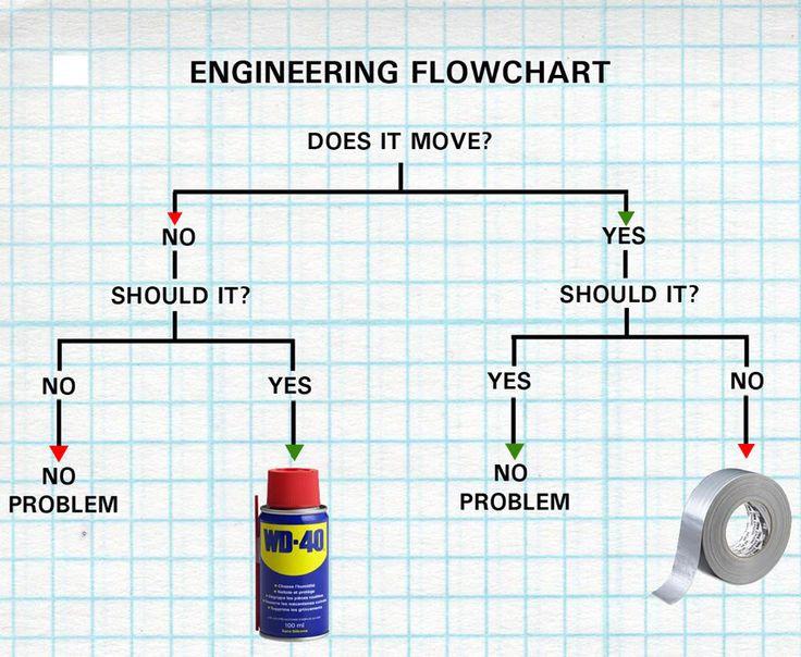
The following image gives a funny example of how decision trees work:
Yet, in machine learning we don’t want to build the decision tree ourselves but let the machine do it (all used packages can be installed from CRAN):
library(OneR)
library(rpart)
library(rpart.plot)

pm_model <- rpart(Machine.failure ~ Type + Air.temperature..K. + Process.temperature..K. + Rotational.speed..rpm. + Torque..Nm. + Tool.wear..min., data = machine_data)
rpart.plot(pm_model, type = 5, extra = 0, box. Palette = "Grays")
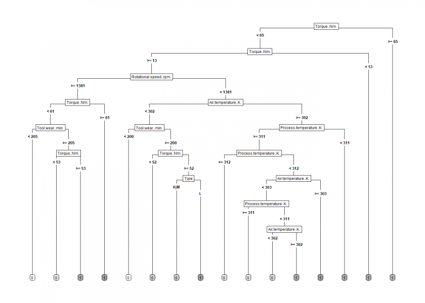
The decision tree is quite convoluted but should still be interpretable by an expert. We used the whole dataset to build it. To get an idea of how well it will perform in real life we train it with a 70% sample of the data and test it with the remaining 30%:
set. Seed(12)
random <- sample(1:nrow(machine_data), 0.7 * nrow(machine_data))
machine_data_train <- machine_data[random, ]
machine_data_test <- machine_data[-random, ]

pm_model <- rpart(Machine.failure ~ Type + Air.temperature..K. + Process.temperature..K. + Rotational.speed..rpm. + Torque..Nm. + Tool.wear..min., data = machine_data_train)
prediction <- predict(pm_model, machine_data_test, type = "class")
eval_model(prediction, machine_data_test)
##
## Confusion matrix (absolute):
##           Actual
## Prediction    0    1  Sum
##        0   2895   35 2930
##        1      9   61   70
##        Sum 2904   96 3000
##
## Confusion matrix (relative):
##           Actual
## Prediction    0    1  Sum
##        0   0.96 0.01 0.98
##        1   0.00 0.02 0.02
##        Sum 0.97 0.03 1.00
##
## Accuracy:
## 0.9853 (2956/3000)
##
## Error rate:
## 0.0147 (44/3000)
##
## Error rate reduction (vs. base rate):
## 0.5417 (p-value = 1.441e-09)
The accuracy is now up to nearly 99%, a statistically significant error rate reduction of more than 50% compared to our naive (and not very helpful) model from above.
So, we achieved both goals, interpretability and high accuracy, with our decision tree – quite an impressive feat!
More and more companies aspire to switch from conventional to predictive maintenance, I myself was a principal consultant for a big project in a multinational chemical industry group.
If you have experience in this fascinating area, please share some examples with us in the comments!
One thought on “Learning Data Science: Predictive Maintenance with Decision Trees”