Pseudo-Randomness: Creating Fake Noise

In data science, we try to find, sometimes well-hidden, patterns (= signal) in often seemingly random data (= noise). Pseudo-Random Number Generators (PRNG) try to do the opposite: hiding a deterministic data generating process (= signal) by making it look like randomness (= noise). If you want to understand some basics behind the scenes of this fascinating topic, read on!

In many an application, we rely on randomness. The problem is that a Turing machine, the theoretical foundation of every computer, knows no randomness. We need to create something that looks like randomness out of determinism. There are at least three questions hidden within:

1. What is true randomness?
2. What does “look like” mean in this context?
3. Which data generating processes can be used in practice?

As you can imagine this is a huge topic and you can think about and do research on those topics for the rest of your remaining life. So, we leave number one to philosophy (and perhaps to a later post), will give a few hints on number two, and will foremost encounter a practical algorithm that is actually used to achieve number three and program it in R!

Normally users don’t think much about these topics but start to wonder what the set.seed() function is for. When I start to explain to my students that you can reproduce the exact same sequence of random numbers by setting a certain seed they mostly look at me as if I had lost my mind. The concept “exact same sequence of random numbers” just doesn’t make sense to them… and yet it is true:

set.seed(42); (u1 <- runif(30))
##  [1] 0.91480604 0.93707541 0.28613953 0.83044763 0.64174552 0.51909595
##  [7] 0.73658831 0.13466660 0.65699229 0.70506478 0.45774178 0.71911225
## [13] 0.93467225 0.25542882 0.46229282 0.94001452 0.97822643 0.11748736
## [19] 0.47499708 0.56033275 0.90403139 0.13871017 0.98889173 0.94666823
## [25] 0.08243756 0.51421178 0.39020347 0.90573813 0.44696963 0.83600426

set.seed(42); (u2 <- runif(30))
##  [1] 0.91480604 0.93707541 0.28613953 0.83044763 0.64174552 0.51909595
##  [7] 0.73658831 0.13466660 0.65699229 0.70506478 0.45774178 0.71911225
## [13] 0.93467225 0.25542882 0.46229282 0.94001452 0.97822643 0.11748736
## [19] 0.47499708 0.56033275 0.90403139 0.13871017 0.98889173 0.94666823
## [25] 0.08243756 0.51421178 0.39020347 0.90573813 0.44696963 0.83600426

identical(u1, u2)
## [1] TRUE

One way to illustrate this idea is to build a pseudorandom number generator (PRNG) ourselves. An especially simple one is a so-called Linear Congruential Generator (LCG). To generate a new random number you use this simple recurrence relation:

   

is our new random number, which is created out of the random number before that (or the seed to create the first random number). , and are predefined values and is just the remainder of the division by (%% in R).

The mathematical theory of how to choose good values for , and is beyond this post. “Good” means that the generated random numbers actually “look” random. Some important criteria for that are:

1. Uniformity of distribution for large quantities of generated numbers.
2. Uncorrelatedness of successive values.
3. No repetion of sequences of numbers.

Those are ideals no pseudorandom generator can reach but some are better than others in this regard. Ours is not particularly great but simple and relatively fast, so without further ado, we are going to build it in R. Actually we will build two different versions based on a task given by Rosetta Code, where I also posted my solution (for details see: Rosetta Code: Linear congruential generator). To be able to cope with very big integers that can occur during the intermediate steps of the calculation we use the gmp package (on CRAN):

library(gmp) # for big integers
## 
## Attaching package: 'gmp'
## The following objects are masked from 'package:base':
## 
##     %*%, apply, crossprod, matrix, tcrossprod

rand_BSD <- function(n = 1) {
  a <- as.bigz(1103515245)
  c <- as.bigz(12345)
  m <- as.bigz(2^31)
  x <- rep(as.bigz(0), n)
  x[1] <- (a * as.bigz(seed) + c) %% m
  i <- 1
  while (i < n) {
    x[i+1] <- (a * x[i] + c) %% m
    i <- i + 1
  }
  as.integer(x)
}

seed <- 0
rand_BSD(10)
##  [1]      12345 1406932606  654583775 1449466924  229283573 1109335178
##  [7] 1051550459 1293799192  794471793  551188310

rand_MS <- function(n = 1) {
  a <- as.bigz(214013)
  c <- as.bigz(2531011)
  m <- as.bigz(2^31)
  x <- rep(as.bigz(0), n)
  x[1] <- (a * as.bigz(seed) + c) %% m
  i <- 1
  while (i < n) {
    x[i+1] <- (a * x[i] + c) %% m
    i <- i + 1
  }
  as.integer(x / 2^16)
}

seed <- 0
rand_MS(10)
##  [1]    38  7719 21238  2437  8855 11797  8365 32285 10450 30612

In the second version (used by Microsoft) the results are divided by 65536 so that the created numbers lie in a range between 0 and 32767.

To create random numbers between 0 and 1 we just divide by 32767:

runif_MS <- function(n = 1) {
  rand_MS(n) / 32767
}

boxplot(runif_MS(1000))

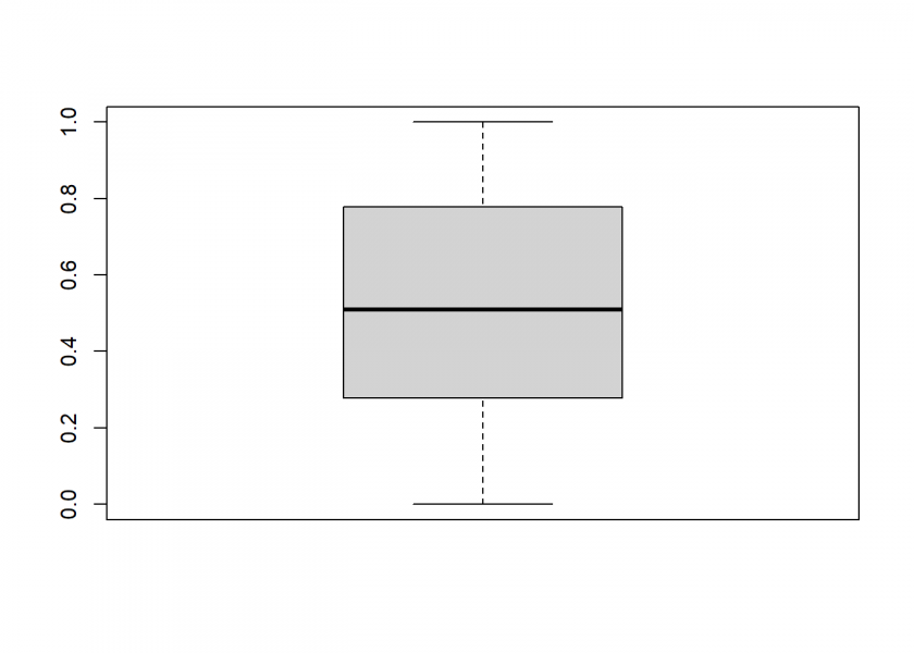
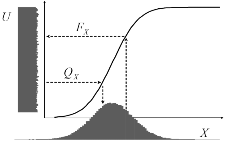
This seems to work pretty well. Sometimes we don’t want uniform random numbers but another distribution, most often normally distributed ones. The following illustration from Attilio Meucci’s excellent book “Risk and Asset Allocation” shows that this could easily be done by a mathematical transformation via the quantile function (here ) of the respective distribution:

In R:

rnorm_MS <- function(n = 1) {
  qnorm(runif_MS(n))
}

rand_NV <- rnorm_MS(2000)
hist(rand_NV)

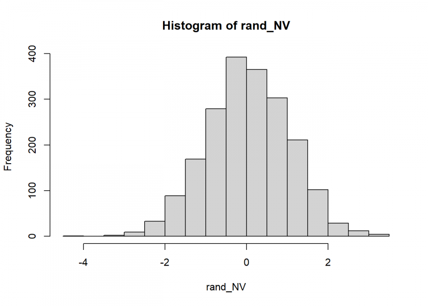
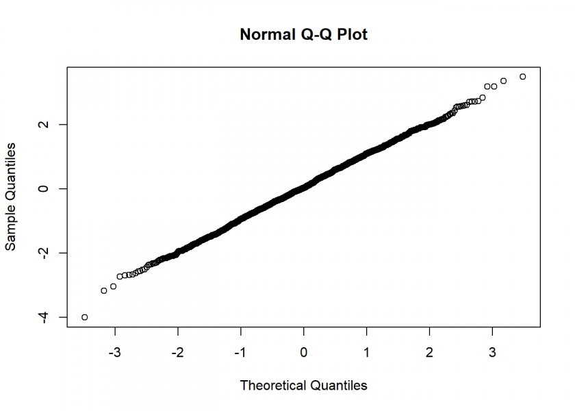
Not too bad… the Q-Q Plot, which compares the generates numbers to the real normal distribution, corroborates this:

qqnorm(rand_NV)

I hope you enjoyed our little journey from determinism via uniform to normally distributed (pseudo-)random numbers… in case you are still thinking about the question at the beginning (What is true randomness?), I have something for you to end this post: