

One of the problems of navigating an autonomous car through a city is to extract robust signals in the face of all the noise that is present in the different sensors. Just taking something like an arithmetic mean of all the data points could possibly end in a catastrophe: if a part of a wall looks similar to the street and the algorithm calculates an average trajectory of the two this would end in leaving the road and possibly crashing into pedestrians. So we need some robust algorithm to get rid of the noise. The area of statistics that especially deals with such problems is called robust statistics and the methods used therein robust estimation.
Now, one of the problems is that one doesn’t know what is signal and what is noise. The big idea behind RANSAC (short for RAndom SAmple Consensus) is to get rid of outliers by basically taking as many points as possible which form a well-defined region and leaving out the others. It does that iteratively, similar to the famous k-means algorithm (the topic of one of the upcoming posts, so stay tuned…).
To really understand how RANSAC works we will now build it with R. We will take a simple linear regression as an example and make it robust against outliers.
For educational purposes we will do this step by step:
- Understanding the general outline of the algorithm.
- Looking at the steps in more detail.
- Expressing the steps in pseudocode.
- Translating this into R!
Conveniently enough Wikipedia gives a good outline of the algorithm and even provides us with the very clear pseudocode which will serve as the basis for our own R implementation (the given Matlab code is not very good in my opinion and has nothing to do with the pseudocode):
The RANSAC algorithm is essentially composed of two steps that are iteratively repeated:
- In the first step, a sample subset containing minimal data items is randomly selected from the input dataset. A fitting model and the corresponding model parameters are computed using only the elements of this sample subset. The cardinality of the sample subset is the smallest sufficient to determine the model parameters.
- In the second step, the algorithm checks which elements of the entire dataset are consistent with the model instantiated by the estimated model parameters obtained from the first step. A data element will be considered as an outlier if it does not fit the fitting model instantiated by the set of estimated model parameters within some error threshold that defines the maximum deviation attributable to the effect of noise. The set of inliers obtained for the fitting model is called consensus set. The RANSAC algorithm will iteratively repeat the above two steps until the obtained consensus set in certain iteration has enough inliers.
In more detail:
RANSAC achieves its goal by repeating the following steps:
- Select a random subset of the original data. Call this subset the hypothetical inliers.
- A model is fitted to the set of hypothetical inliers.
- All other data are then tested against the fitted model. Those points that fit the estimated model well, according to some model-specific loss function, are considered as part of the consensus set.
- The estimated model is reasonably good if sufficiently many points have been classified as part of the consensus set.
- Afterwards, the model may be improved by reestimating it using all members of the consensus set.
This procedure is repeated a fixed number of times, each time producing either a model which is rejected because too few points are part of the consensus set, or a refined model together with a corresponding consensus set size. In the latter case, we keep the refined model if its consensus set is larger than the previously saved model.
Now, this can be expressed in pseudocode:
Given:
    data - a set of observed data points
    model - a model that can be fitted to data points
    n - minimum number of data points required to fit the model
    k - maximum number of iterations allowed in the algorithm
    t - threshold value to determine when a data point fits a model
    d - number of close data points required to assert that a model fits well to data

Return:
    bestfit - model parameters which best fit the data (or nul if no good model is found)

iterations = 0
bestfit = nul
besterr = something really large
while iterations < k {
    maybeinliers = n randomly selected values from data
    maybemodel = model parameters fitted to maybeinliers
    alsoinliers = empty set
    for every point in data not in maybeinliers {
        if point fits maybemodel with an error smaller than t
             add point to alsoinliers
    }
    if the number of elements in alsoinliers is > d {
        % this implies that we may have found a good model
        % now test how good it is
        bettermodel = model parameters fitted to all points in maybeinliers and alsoinliers
        thiserr = a measure of how well model fits these points
        if thiserr < besterr {
            bestfit = bettermodel
            besterr = thiserr
        }
    }
    increment iterations
}
return bestfit
It is quite easy to convert this into valid R code (as a learner of R you should try it yourself before looking at my solution!):
ransac <- function(data, n, k, t, d) {
  iterations <- 0
  bestfit <- NULL
  besterr <- 1e5
  while (iterations < k) {
    maybeinliers <- sample(nrow(data), n)
    maybemodel <- lm(y ~ x, data = data, subset = maybeinliers)
    alsoinliers <- NULL
    for (point in setdiff(1:nrow(data), maybeinliers)) {
      if (abs(maybemodel$coefficients[2]*data[point, 1] - data[point, 2] + maybemodel$coefficients[1])/(sqrt(maybemodel$coefficients[2] + 1)) < t)
        alsoinliers <- c(alsoinliers, point)
    }
    if (length(alsoinliers) > d) {
      bettermodel <- lm(y ~ x, data = data, subset = c(maybeinliers, alsoinliers))
      thiserr <- summary(bettermodel)$sigma
      if (thiserr < besterr) {
        bestfit <- bettermodel
        besterr <- thiserr
      }
    }
    iterations <- iterations + 1
  }
  bestfit
}
We now test this with some sample data:
data <- read.csv("data/RANSAC.csv")
plot(data)
abline(lm(y ~ x, data = data))
set.seed(3141)
abline(ransac(data, n = 10, k = 10, t = 0.5, d = 10), col = "blue")
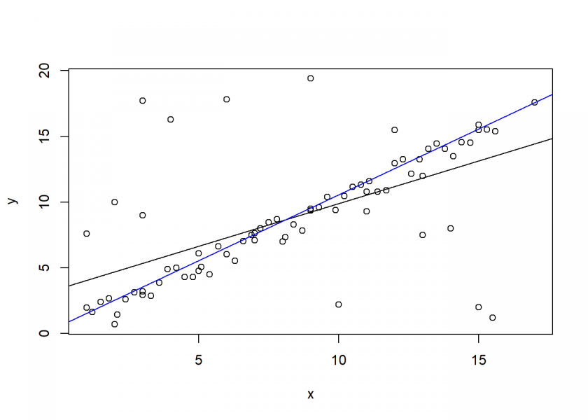
The black line is a plain vanilla linear regression, the blue line is the RANSAC-enhanced version. As you can see: no more crashing into innocent pedestrians. 🙂
how did you derive your hyperparameters?
It is a combination of experimental evaluation and some rules of thumb (based on statistical considerations), as a starting point see: https://en.wikipedia.org/wiki/Random_sample_consensus#Parameters.
Could you justify the choice f the loss function?