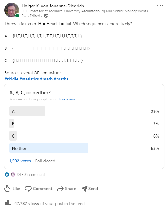
 Some time ago I conducted a poll on LinkedIn that quickly went viral. I asked which of three different coin tossing sequences were more likely and I received exactly 1,592 votes! Nearly 48,000 people viewed it and more than 80 comments are under the post (you need a LinkedIn account to fully see it here: LinkedIn Coin Tossing Poll).
In this post I will give the solution with some background explanation, so read on!
Please have a look at the original question and the final result:

The majority (exactly 1,000 people!) got it right, all of these sequences are equally likely. But why are they? To answer probability-related questions there are basically three approaches: analytically, by simulation, or by listing all possible outcomes. We will go for the third method because the resulting set is still small enough to be efficiently handled by R, it is very intuitive, and it gives us exact results which we can then compare to the analytical solution.
Let us first define our three sequences in R and then create a big matrix with all possible sequences:
A <- c("H", "T", "H", "T", "H", "T", "H", "T", "H", "T", "T", "H", "T", "H", "H", "T", "T", "T", "H")
B <- c(rep("H", 19))
C <- c(rep("H", 10), rep("T", 9))

M <- as.matrix(expand.grid(rep(list(c("H", "T")), 19)))
head(M, 10)
##       Var1 Var2 Var3 Var4 Var5 Var6 Var7 Var8 Var9 Var10 Var11 Var12 Var13
##  [1,] "H"  "H"  "H"  "H"  "H"  "H"  "H"  "H"  "H"  "H"   "H"   "H"   "H"
##  [2,] "T"  "H"  "H"  "H"  "H"  "H"  "H"  "H"  "H"  "H"   "H"   "H"   "H"
##  [3,] "H"  "T"  "H"  "H"  "H"  "H"  "H"  "H"  "H"  "H"   "H"   "H"   "H"
##  [4,] "T"  "T"  "H"  "H"  "H"  "H"  "H"  "H"  "H"  "H"   "H"   "H"   "H"
##  [5,] "H"  "H"  "T"  "H"  "H"  "H"  "H"  "H"  "H"  "H"   "H"   "H"   "H"
##  [6,] "T"  "H"  "T"  "H"  "H"  "H"  "H"  "H"  "H"  "H"   "H"   "H"   "H"
##  [7,] "H"  "T"  "T"  "H"  "H"  "H"  "H"  "H"  "H"  "H"   "H"   "H"   "H"
##  [8,] "T"  "T"  "T"  "H"  "H"  "H"  "H"  "H"  "H"  "H"   "H"   "H"   "H"
##  [9,] "H"  "H"  "H"  "T"  "H"  "H"  "H"  "H"  "H"  "H"   "H"   "H"   "H"
## [10,] "T"  "H"  "H"  "T"  "H"  "H"  "H"  "H"  "H"  "H"   "H"   "H"   "H"
##       Var14 Var15 Var16 Var17 Var18 Var19
##  [1,] "H"   "H"   "H"   "H"   "H"   "H"
##  [2,] "H"   "H"   "H"   "H"   "H"   "H"
##  [3,] "H"   "H"   "H"   "H"   "H"   "H"
##  [4,] "H"   "H"   "H"   "H"   "H"   "H"
##  [5,] "H"   "H"   "H"   "H"   "H"   "H"
##  [6,] "H"   "H"   "H"   "H"   "H"   "H"
##  [7,] "H"   "H"   "H"   "H"   "H"   "H"
##  [8,] "H"   "H"   "H"   "H"   "H"   "H"
##  [9,] "H"   "H"   "H"   "H"   "H"   "H"
## [10,] "H"   "H"   "H"   "H"   "H"   "H"

tail(M, 10)
##           Var1 Var2 Var3 Var4 Var5 Var6 Var7 Var8 Var9 Var10 Var11 Var12 Var13
## [524279,] "H"  "T"  "T"  "H"  "T"  "T"  "T"  "T"  "T"  "T"   "T"   "T"   "T"
## [524280,] "T"  "T"  "T"  "H"  "T"  "T"  "T"  "T"  "T"  "T"   "T"   "T"   "T"
## [524281,] "H"  "H"  "H"  "T"  "T"  "T"  "T"  "T"  "T"  "T"   "T"   "T"   "T"
## [524282,] "T"  "H"  "H"  "T"  "T"  "T"  "T"  "T"  "T"  "T"   "T"   "T"   "T"
## [524283,] "H"  "T"  "H"  "T"  "T"  "T"  "T"  "T"  "T"  "T"   "T"   "T"   "T"
## [524284,] "T"  "T"  "H"  "T"  "T"  "T"  "T"  "T"  "T"  "T"   "T"   "T"   "T"
## [524285,] "H"  "H"  "T"  "T"  "T"  "T"  "T"  "T"  "T"  "T"   "T"   "T"   "T"
## [524286,] "T"  "H"  "T"  "T"  "T"  "T"  "T"  "T"  "T"  "T"   "T"   "T"   "T"
## [524287,] "H"  "T"  "T"  "T"  "T"  "T"  "T"  "T"  "T"  "T"   "T"   "T"   "T"
## [524288,] "T"  "T"  "T"  "T"  "T"  "T"  "T"  "T"  "T"  "T"   "T"   "T"   "T"
##           Var14 Var15 Var16 Var17 Var18 Var19
## [524279,] "T"   "T"   "T"   "T"   "T"   "T"
## [524280,] "T"   "T"   "T"   "T"   "T"   "T"
## [524281,] "T"   "T"   "T"   "T"   "T"   "T"
## [524282,] "T"   "T"   "T"   "T"   "T"   "T"
## [524283,] "T"   "T"   "T"   "T"   "T"   "T"
## [524284,] "T"   "T"   "T"   "T"   "T"   "T"
## [524285,] "T"   "T"   "T"   "T"   "T"   "T"
## [524286,] "T"   "T"   "T"   "T"   "T"   "T"
## [524287,] "T"   "T"   "T"   "T"   "T"   "T"
## [524288,] "T"   "T"   "T"   "T"   "T"   "T"
We see that there are exactly 524,288 sequences. That is because there are two possibilities for the first coin times two possibilities for the second times… and so on, which give 2^19 = 524,288 sequences altogether
Now let us find out how often each sequence appears:
sum(colSums(t(M) == A) == 19) # how many possibilities are exactly equal to A
## [1] 1

sum(colSums(t(M) == B) == 19)
## [1] 1

sum(colSums(t(M) == C) == 19)
## [1] 1
Each sequence appears exactly once. The probability for each sequence therefore is…
1 / nrow(M)
## [1] 1.907349e-06
…which is exactly 1/2^19 for all three cases because the coin tosses are independent of each other.
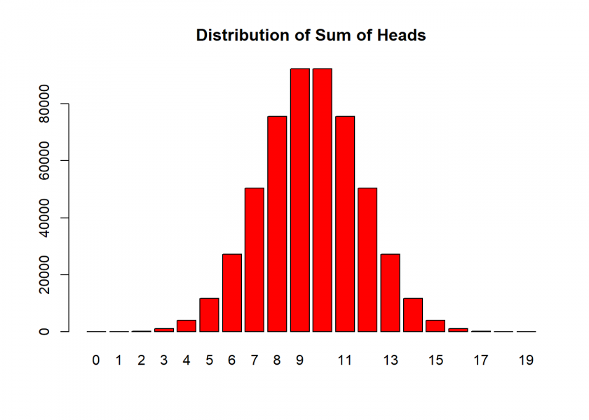
But why do so many people, also some renowned data scientists and even colleagues of mine, chose A? My guess is that they confuse the actual sequences with some derived feature, like the sum of heads. Counting the number of heads in each sequence shows a completely different picture, which can also be derived analytically by using the binomial distribution:
tab <- rbind(counting = table(colSums(t(M) == B)), binomial = dbinom(0:19, 19, 0.5) * nrow(M))
tab
##          0  1   2   3    4     5     6     7     8     9    10    11    12
## counting 1 19 171 969 3876 11628 27132 50388 75582 92378 92378 75582 50388
## binomial 1 19 171 969 3876 11628 27132 50388 75582 92378 92378 75582 50388
##             13    14   15  16  17 18 19
## counting 27132 11628 3876 969 171 19  1
## binomial 27132 11628 3876 969 171 19  1

barplot(tab[1, ], col = "red", main = "Distribution of Sum of Heads")

So, the probability of seeing some mix of “H” and “T” is much higher than seeing only heads or only tails… but “some mix” is something completely different than an exact sequence like A (which all have the same probability as we just saw).
The distribution suspiciously looks like a normal distribution and the reason for this is the Central Limit Theorem (CLT), which was the topic of another post: The Central Limit Theorem (CLT): From Perfect Symmetry to the Normal Distribution.
I hope that this clarifies the issue and I look forward to your comments below.
P.S.: There might be even another misconception at play here, especially when you look at the run of heads and tails and how they change in sequence C. It has to do with the so-called Law of Large Numbers and will be the topic of our post next week, so stay tuned!

Dear Holger,
thanks for another interesting post. As the supposed bias in human perception of randomness is a highly controversial topic in psychology, I suggest looking at the other side of the coin as well:
Your enumeration of possible cases relies on the implicit premise that a fair coin is tossed exactly 19 times and the probability of this event behaves exactly as projected by an idealized probability calculus (or an infinite number of tosses).
However, if we assume that humans are more likely to experience many tosses of finite length, the more irregular series A actually appears more frequently than the regular series B. The details of this argument are spelled out in the following paper:
Hahn, U., & Warren, P. A. (2009). Perceptions of randomness: Why three heads are better than four.
Psychological Review, 116(2), 454–461. https://doi.org/10.1037/a0015241
Its conclusion reads: “the case against lay intuitions about randomness needs to be reopened. Both how and how well people identify random sources are questions in need of reevaluation.” (p. 460).
In my experience, people always find demonstrations of alleged biases more appealing than the scientific analysis why things are perceived as they are. But finding out that people actually have good reasons for their seemingly irrational perceptions can also be fun.
Best,
Hans
PS: Implementations of both the pro- and contra-bias arguments are available at
https://bookdown.org/hneth/i2ds/15-5-sims-ex.html#sims:ex-coin-toss
(I took the liberty to add a link to your post in the combinatorial description of the problem.)