
We already saw the power of the OneR package in the preceding post, One Rule (OneR) Machine Learning Classification in under One Minute. Here we want to give some more examples to gain some fascinating, often counter-intuitive, insights.
Shirin Glander of Muenster University tested the OneR package with data from the World Happiness Report to find out what makes people happy: https://shiring.github.io/machine_learning/2017/04/23/one_r.
The whole analysis is very sophisticated so I present a simplified approach here. Have a look at the following code:
library(OneR)
data <- read.csv("data/2016.csv", sep = ",", header = TRUE)
data$Happiness.Score <- bin(data$Happiness.Score, nbins = 3, labels = c("low", "middle", "high"), method = "content")
data <- maxlevels(data) # removes all columns that have more than 20 levels (Country)
data <- optbin(formula = Happiness.Score ~., data = data, method = "infogain")
data <- data[ , -(1:4)] # remove columns with redundant data
model <- OneR(formula = Happiness.Score ~., data = data, verbose = TRUE)
##
##     Attribute                     Accuracy
## 1 * Economy..GDP.per.Capita.      71.97%
## 2   Health..Life.Expectancy.      70.06%
## 3   Family                        65.61%
## 4   Dystopia.Residual             59.87%
## 5   Freedom                       57.32%
## 6   Trust..Government.Corruption. 55.41%
## 7   Generosity                    47.13%
## ---
## Chosen attribute due to accuracy
## and ties method (if applicable): '*'
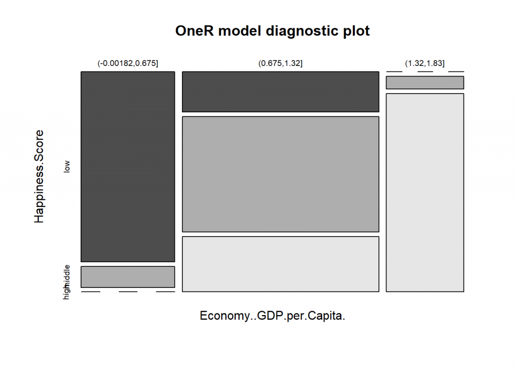
summary(model)
##
## Call:
## OneR.formula(formula = Happiness.Score ~ ., data = data, verbose = TRUE)
##
## Rules:
## If Economy..GDP.per.Capita. = (-0.00182,0.675] then Happiness.Score = low
## If Economy..GDP.per.Capita. = (0.675,1.32]     then Happiness.Score = middle
## If Economy..GDP.per.Capita. = (1.32,1.83]      then Happiness.Score = high
##
## Accuracy:
## 113 of 157 instances classified correctly (71.97%)
##
## Contingency table:
##                Economy..GDP.per.Capita.
## Happiness.Score (-0.00182,0.675] (0.675,1.32] (1.32,1.83] Sum
##          low                * 36           16           0  52
##          middle                4         * 46           2  52
##          high                  0           22        * 31  53
##          Sum                  40           84          33 157
## ---
## Maximum in each column: '*'
##
## Pearson's Chi-squared test:
## X-squared = 130.99, df = 4, p-value < 2.2e-16
plot(model)
prediction <- predict(model, data)
eval_model(prediction, data)
##
## Confusion matrix (absolute):
##           Actual
## Prediction high low middle Sum
##     high     31   0      2  33
##     low       0  36      4  40
##     middle   22  16     46  84
##     Sum      53  52     52 157
##
## Confusion matrix (relative):
##           Actual
## Prediction high  low middle  Sum
##     high   0.20 0.00   0.01 0.21
##     low    0.00 0.23   0.03 0.25
##     middle 0.14 0.10   0.29 0.54
##     Sum    0.34 0.33   0.33 1.00
##
## Accuracy:
## 0.7197 (113/157)
##
## Error rate:
## 0.2803 (44/157)
##
## Error rate reduction (vs. base rate):
## 0.5769 (p-value < 2.2e-16)
As you can see we get more than 70% accuracy with three rules based on GDP per capita. So it seems that money CAN buy happiness after all!
Dr. Glander comes to the following conclusion:
All in all, based on this example, I would confirm that OneR models do indeed produce sufficiently accurate models for setting a good baseline. OneR was definitely faster than random forest, gradient boosting and neural nets. However, the latter were more complex models and included cross-validation.
If you prefer an easy to understand model that is very simple, OneR is a very good way to go. You could also use it as a starting point for developing more complex models with improved accuracy.
When looking at feature importance across models, the feature OneR chose – Economy/GDP per capita – was confirmed by random forest, gradient boosting trees and neural networks as being the most important feature. This is in itself an interesting conclusion! Of course, this correlation does not tell us that there is a direct causal relationship between money and happiness, but we can say that a country’s economy is the best individual predictor for how happy people tend to be.
A well known reference data set is the titanic data set which gives all kind of additional information on the passengers of the titanic and whether they survived the tragedy. We can conveniently use the titanic package from CRAN to get access to the data set. Have a look at the following code:
library(titanic)
data <- bin(maxlevels(titanic_train), na.omit = FALSE)
model <- OneR(Survived ~., data = data, verbose = TRUE)
## Warning in OneR.data.frame(x = data, ties.method = ties.method, verbose =
## verbose, : data contains unused factor levels
##
##     Attribute   Accuracy
## 1 * Sex         78.68%
## 2   Pclass      67.9%
## 3   Fare        64.42%
## 4   Embarked    63.86%
## 5   Age         62.74%
## 6   Parch       61.73%
## 7   PassengerId 61.62%
## 7   SibSp       61.62%
## ---
## Chosen attribute due to accuracy
## and ties method (if applicable): '*'
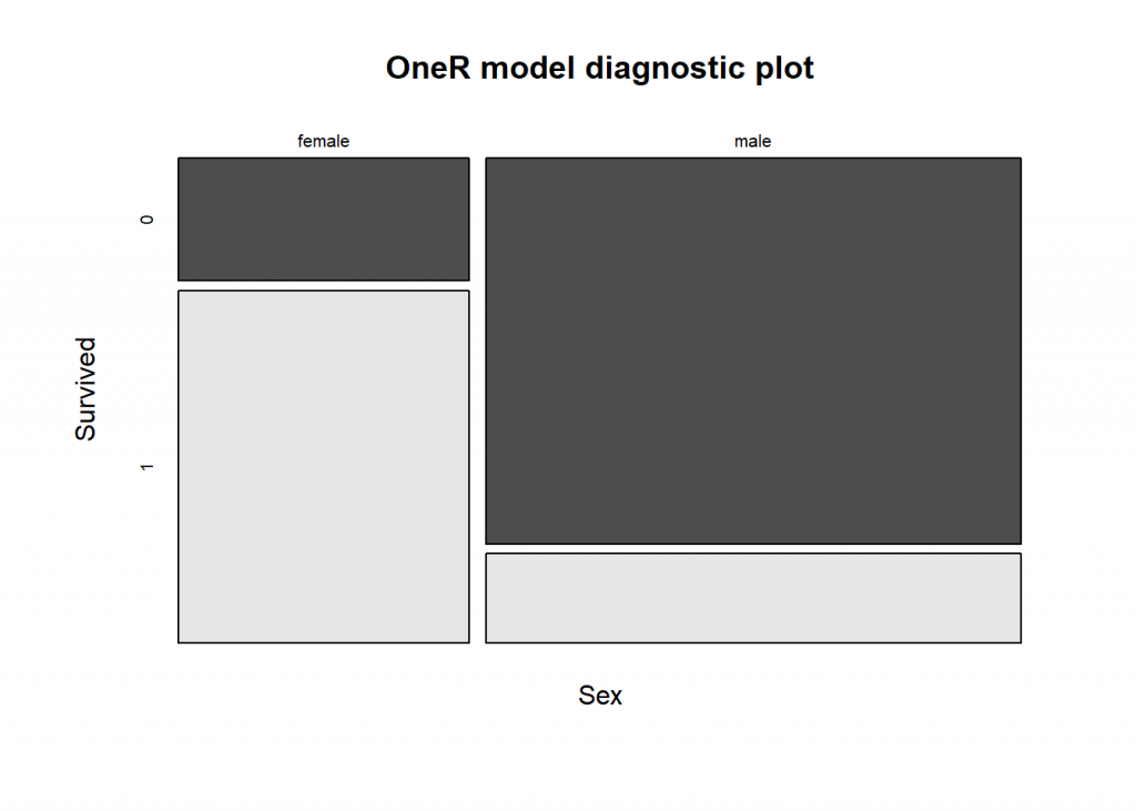
summary(model)
##
## Call:
## OneR.formula(formula = Survived ~ ., data = data, verbose = TRUE)
##
## Rules:
## If Sex = female then Survived = 1
## If Sex = male   then Survived = 0
##
## Accuracy:
## 701 of 891 instances classified correctly (78.68%)
##
## Contingency table:
##         Sex
## Survived female  male Sum
##      0       81 * 468 549
##      1    * 233   109 342
##      Sum    314   577 891
## ---
## Maximum in each column: '*'
##
## Pearson's Chi-squared test:
## X-squared = 260.72, df = 1, p-value < 2.2e-16
plot(model)
prediction <- predict(model, data)
eval_model(prediction, data$Survived)
##
## Confusion matrix (absolute):
##           Actual
## Prediction   0   1 Sum
##        0   468 109 577
##        1    81 233 314
##        Sum 549 342 891
##
## Confusion matrix (relative):
##           Actual
## Prediction    0    1  Sum
##        0   0.53 0.12 0.65
##        1   0.09 0.26 0.35
##        Sum 0.62 0.38 1.00
##
## Accuracy:
## 0.7868 (701/891)
##
## Error rate:
## 0.2132 (190/891)
##
## Error rate reduction (vs. base rate):
## 0.4444 (p-value < 2.2e-16)
So, somewhat contrary to popular belief, it were not necessarily the rich that survived but the women!
A more challenging data set is one about the quality of red wine (https://archive.ics.uci.edu/ml/datasets/Wine+Quality), have a look at the following code:
data <- read.csv("data/winequality-red.csv", header = TRUE, sep = ";")
data <- optbin(data, method = "infogain")
## Warning in optbin.data.frame(data, method = "infogain"): target is numeric
model <- OneR(data, verbose = TRUE)
##
##     Attribute            Accuracy
## 1 * alcohol              56.1%
## 2   sulphates            51.22%
## 3   volatile.acidity     50.59%
## 4   total.sulfur.dioxide 48.78%
## 5   density              47.22%
## 6   citric.acid          46.72%
## 7   chlorides            46.47%
## 8   free.sulfur.dioxide  44.47%
## 9   fixed.acidity        43.96%
## 10  residual.sugar       43.46%
## 11  pH                   43.21%
## ---
## Chosen attribute due to accuracy
## and ties method (if applicable): '*'
summary(model)
##
## Call:
## OneR.data.frame(x = data, verbose = TRUE)
##
## Rules:
## If alcohol = (8.39,8.45] then quality = 3
## If alcohol = (8.45,10]   then quality = 5
## If alcohol = (10,11]     then quality = 6
## If alcohol = (11,12.5]   then quality = 6
## If alcohol = (12.5,14.9] then quality = 6
##
## Accuracy:
## 897 of 1599 instances classified correctly (56.1%)
##
## Contingency table:
##        alcohol
## quality (8.39,8.45] (8.45,10] (10,11] (11,12.5] (12.5,14.9]  Sum
##     3           * 1         5       4         0           0   10
##     4             0        28      13        11           1   53
##     5             0     * 475     156        41           9  681
##     6             1       216   * 216     * 176        * 29  638
##     7             0        19      53       104          23  199
##     8             0         2       2         6           8   18
##     Sum           2       745     444       338          70 1599
## ---
## Maximum in each column: '*'
##
## Pearson's Chi-squared test:
## X-squared = 546.64, df = 20, p-value < 2.2e-16
prediction <- predict(model, data)
eval_model(prediction, data, zero.print = ".")
##
## Confusion matrix (absolute):
##           Actual
## Prediction    3    4    5    6    7    8  Sum
##        3      1    .    .    1    .    .    2
##        4      .    .    .    .    .    .    .
##        5      5   28  475  216   19    2  745
##        6      4   25  206  421  180   16  852
##        7      .    .    .    .    .    .    .
##        8      .    .    .    .    .    .    .
##        Sum   10   53  681  638  199   18 1599
##
## Confusion matrix (relative):
##           Actual
## Prediction    3    4    5    6    7    8  Sum
##        3      .    .    .    .    .    .    .
##        4      .    .    .    .    .    .    .
##        5      . 0.02 0.30 0.14 0.01    . 0.47
##        6      . 0.02 0.13 0.26 0.11 0.01 0.53
##        7      .    .    .    .    .    .    .
##        8      .    .    .    .    .    .    .
##        Sum 0.01 0.03 0.43 0.40 0.12 0.01 1.00
##
## Accuracy:
## 0.561 (897/1599)
##
## Error rate:
## 0.439 (702/1599)
##
## Error rate reduction (vs. base rate):
## 0.2353 (p-value < 2.2e-16)
That is an interesting result, isn’t it: the more alcohol the higher the perceived quality!
We end this post with an unconventional use case for OneR: finding the best move in a strategic game, i.e. tic-tac-toe. We use a dataset with all possible board configurations at the end of such games, have a look at the following code:
data <- read.csv("https://archive.ics.uci.edu/ml/machine-learning-databases/tic-tac-toe/tic-tac-toe.data", header = FALSE)
names(data) <- c("top-left-square", "top-middle-square", "top-right-square", "middle-left-square", "middle-middle-square", "middle-right-square", "bottom-left-square", "bottom-middle-square", "bottom-right-square", "Class")
model <- OneR(data, verbose = TRUE)
##
##     Attribute            Accuracy
## 1 * middle-middle-square 69.94%
## 2   top-left-square      65.34%
## 2   top-middle-square    65.34%
## 2   top-right-square     65.34%
## 2   middle-left-square   65.34%
## 2   middle-right-square  65.34%
## 2   bottom-left-square   65.34%
## 2   bottom-middle-square 65.34%
## 2   bottom-right-square  65.34%
## ---
## Chosen attribute due to accuracy
## and ties method (if applicable): '*'
summary(model)
##
## Call:
## OneR.data.frame(x = data, verbose = TRUE)
##
## Rules:
## If middle-middle-square = b then Class = positive
## If middle-middle-square = o then Class = negative
## If middle-middle-square = x then Class = positive
##
## Accuracy:
## 670 of 958 instances classified correctly (69.94%)
##
## Contingency table:
##           middle-middle-square
## Class          b     o     x Sum
##   negative    48 * 192    92 332
##   positive * 112   148 * 366 626
##   Sum        160   340   458 958
## ---
## Maximum in each column: '*'
##
## Pearson's Chi-squared test:
## X-squared = 115.91, df = 2, p-value < 2.2e-16
prediction <- predict(model, data)
eval_model(prediction, data)
##
## Confusion matrix (absolute):
##           Actual
## Prediction negative positive Sum
##   negative      192      148 340
##   positive      140      478 618
##   Sum           332      626 958
##
## Confusion matrix (relative):
##           Actual
## Prediction negative positive  Sum
##   negative     0.20     0.15 0.35
##   positive     0.15     0.50 0.65
##   Sum          0.35     0.65 1.00
##
## Accuracy:
## 0.6994 (670/958)
##
## Error rate:
## 0.3006 (288/958)
##
## Error rate reduction (vs. base rate):
## 0.1325 (p-value = 0.001427)
Perhaps it doesn’t come as a surprise that the middle-middle-square is strategically the most important one – but still it is encouraging to see that OneR comes to the same conclusion.
Thank a lot for this great package.
Any suggestions for visualizing a OneR decision tree object?
Thank you Shani, I really appreciate it!
Well, what do you mean by “decision tree object”? Because basically it is a one-level decision tree the
plotfunction might be the visualization you are looking for?If you have another idea, please share it with me… I am always open to suggestions for improving the package.