

Learning Machines proudly presents a guest post by Martijn Weterings from the Food and Natural Products research group of the Institute of Life Technologies at the University of Applied Sciences of Western Switzerland in Sion.
The topic of this post will be the fitting with the R-package optim. Food? That sounds like a rather unlikely match for writing a post on a blog about quantitative analysis, however, there is a surprising overlap between these disciplinary fields. For example, whether you model the transport of a flavour molecule or transport of a virus, the type of mathematical equations and the ways to treat the data are a lot similar.
This contribution will be split into two parts. In the first part, we pick up on the earlier fitting described in a previous blog-post here (see Epidemiology: How contagious is Novel Coronavirus (2019-nCoV)?). These fits are sometimes difficult to perform. How can we analyse that difficult behaviour and how can we make further improvements? In the second part, we will see that all these efforts to make a nice performing algorithm to perform the fitting is actually not much useful for the current case. Just because we use a mathematical model, which sounds rigorous, does not mean that our conclusions/predictions are trustworthy.
These two parts will be accompanied by the R-script covid.r.
COVID-19: a data epidemic
With the outbreak of COVID-19 one thing that is certain is that never before a virus has gone so much viral on the internet. Especially, a lot of data about the spread of the virus is going around. A large amount of data is available in the form of fancy coronavirus-trackers that look like weather forecasts or overviews of sports results. Many people have started to try predicting the evolution of the epidemiological curve and along with that the reproduction number  , but can this be done with this type of data?
In this blog-post, we describe the fitting of the data with the SIR model and explain the tricky parts of the fitting methodology and how we can mitigate some of the problems that we encounter.
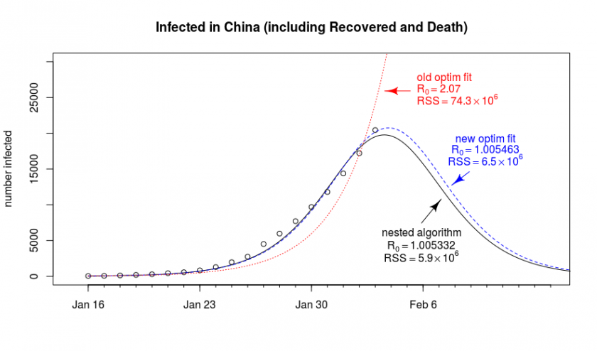
The general problem is that the fitting-algorithm is not always finding it’s way to the best solution. Below is a graph that shows an out of the box fit of the data with the optim package (it’s the one from the previous blog post Epidemiology: How contagious is Novel Coronavirus (2019-nCoV)? ). Next to it, we show a result that is more optimal. Why did we not find this result directly with the optim package?
Why doesn’t the algorithm converge to the optimal solution?
There are two main reasons why the model is not converging well.
Early stopping of the algorithm
The first reason is that the optim algorithm (which is updating model parameters starting from an initial guess and moving towards the optimal solution) is stopping too early before it has found the right solution.
How does the optim package find a solution? The gradient methods used by the optim package find the optimum estimate by repeatedly improving the current estimate and finding a new solution with a lower residual sum of squares (RSS) each time. Gradient methods do this by computing for a small change of the parameters in which direction the RSS will change the fastest and then, in the case of the BFGS method used by the optim package, it computes (via a line search method) where in that direction the lowest value for the RSS is. This is repeated until no further improvement can be made, or when the improvement is below some desired/sufficient minimal level.
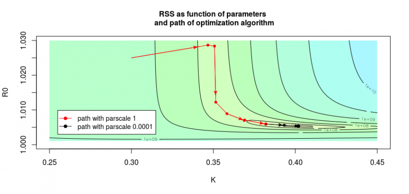
In the two images below we see how the algorithm solves stepwise the fit, for a SIR model that uses the parameters  and
and  (these parameters had been explained in the previous blog post and are repeated in this post below). The images are contour plot (lines) and surface plot (colours) for the value of the RSS as a function of the model parameters. The minimum is around
  and
and  where eventually the algorithm should end.
We see in these images effects that make it difficult for the algorithm to approach the optimum quickly in few steps, or it may even get blocked before that point (also it may end up in a local optimum, which is a bit different case, although we have it here as well and there’s a local optimum with a value for  ).
).
Computation of the gradient If the function that we use for the optimization does not provide an expression for the gradient of the function (which is needed to find the direction of movement) then the optim package will compute this manually by taking the values at nearby points.
How much nearby do these points need to be? The optim package uses the scale of the parameters for this. This scale does not always work out of the box and when it is too large then the algorithm is not making an accurate computation of the gradient.
In the image below we see this by the path taken by the algorithm is shown by the red and black arrows. The red arrows show the path when we do not fine-tune the optimization, the black path shows the path when we reduce the scale of the parameters manually. This is done with the control parameter. In the code of the file covid.R you see this in the function:
OptTemp <- optim(new, RSS2,
                 method = "L-BFGS-B",
                 lower = c(0,1.00001),
                 hessian = TRUE,
                 control = list(parscale = c(10^-4,10^-4),
                                factr = 1))
By using parscale = c(10^-4,10^-4) we let the algorithm compute the gradient at a smaller scale (we could actually also use the ndeps parameter). In addition, we used factr = 1, which is a factor that determines the point when the algorithm stops (in this case when the improvement is less than one times the machine precision).
So by changing the parameter parscale we can often push the algorithm to get closer to the optimal solution.
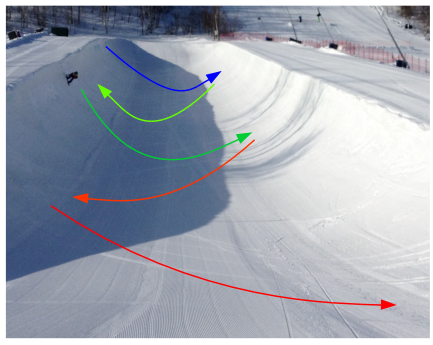
A zigzag path towards the optimum may occur when the surface plot of the RSS has a sort of long stretched valley shape. Then the algorithm is computing a path that moves towards the optimum like a sort of snowboarder on a half-pipe, taking lots of movements along the axis in the direction of the curvature of the half-pipe, and much less movement along the axis downhill towards the bottom.
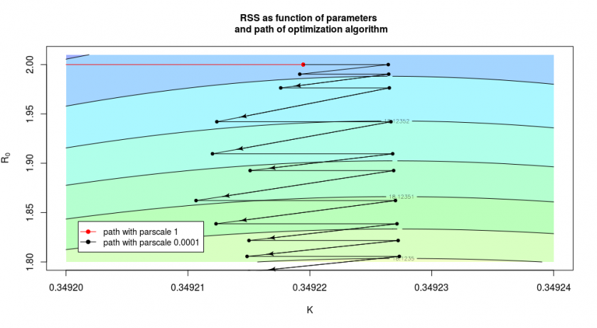
In the case above we had let the algorithm start at and and this was chosen on purpose for the illustration. But we do not always make such a good initial guess. In the image below we see what happens when we had chosen and  as starting condition (note that image should be stretched out along the y-axis due to the different ranges of
  and
and  in which case the change of the RSS is much faster/stronger in the direction left-right than the direction up-down).
The red curve, which shows the result of the algorithm without the fine-tuning, stops already after one step around  where it hits the bottom of the curvature of the valley/half-pipe and is not accurately finding out that there is still a long path/gradient in the other direction. We can improve the situation by changing the
 parscale parameter, in which case the algorithm will more precisely determine the slope and continue it’s path (see the black arrows). But in the direction of the y-axis, it does this only in small steps, so it will only slowly converge to the optimal solution.
We can often improve this situation by changing the relative scale of the parameters, however, in this particular case, it is not easy, because of the L-shape of the ‘valley’ (see the above image). We could change the relative scales of the parameters to improve convergence in the beginning, but then the convergence at the end becomes more difficult.
Ill-conditioned problem
The second reason for the bad convergence behaviour of the algorithm is that the problem is ill-conditioned. That means that a small change of the data will have a large influence on the outcome of the parameter estimates.
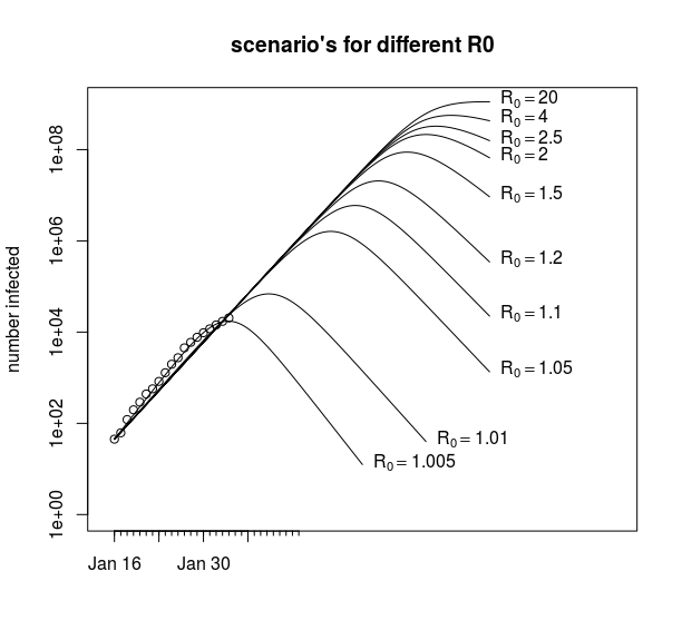
In that case, the data is not very useful to differentiate between different parameters of the model. A large range of variation in the parameters can more or less explain the same data.
An example of this is in the image below, where we see that for different values of R0 we can still fit the data without much difference in the residual sum of squares (RSS). We get every time a value for  around
  to
to  (and the shape of the curve is not much dependent on the value of ).
This value for relates to the initial growth rate. Let’s look at the differential equations to see why variations in have so little effect on the begin of the curve. In terms of the parameters and the equations are now:
![\[\begin{array}{rclc} \frac{dS}{dt} &=& \frac{-S/N R_0}{R_0-1} K I &\\ \\ \frac{dI}{dt} &=& \frac{S/N R_0 - 1}{R_0-1} K I &\underbrace{\approx \,\, KI}_{\llap{\scriptsize\text{if $S/N \approx 1$}}} \\ \\ \frac{dR}{dt} &=& \frac{1}{R_0-1} K I & \end{array}\]](https://blog.ephorie.de/wp-content/ql-cache/quicklatex.com-db11754a226c5395825bc480d62e91b4_l3.png "Rendered by QuickLaTeX.com")
Here we see that, when  is approximately equal to
  (which is the case in the beginning), then we get approximately
  and the beginning of the curve will be approximately exponential.
Thus, for a large range of values of , the beginning of the epidemiological curve will resemble an exponential growth that is independent of the value of . In the opposite direction: when we observe exponential growth (initially) then we can not use this observation to derive a value for .
With these ill-conditioned problems, it is often difficult to get the algorithm to converge to the minimum. This is because changes in some parameter (in our case ) will result in only a small improvement of the RSS and a large range of the parameters have more or less the same RSS.
The error/variance of the parameter estimates
So if small variations in the data occur, due to measurements errors, how much impact will this have on the estimates of the parameters? Here we show the results for two different ways to do determine this. In the file covid.R the execution of the methods will be explained in more detail.
Using an estimate of the Fisher information. We can determine an estimate for (lower bound of) the variance of the parameters by considering the Cramér-Rao bound, which states that the variance of (unbiased) parameter estimates are equal to or larger than the inverse of the Fisher Information matrix. The Fisher information is a matrix with the second-order partial derivatives of the log-likelihood function evaluated at the true parameter values.
The log-likelihood function is this thing:
We do not know this loglikelihood function and it’s dependence on the parameters and because we do not have the true parameter values and also we do not know the variance of the random error of the data points (the  term in the likelihood function). But we can estimate it based on the Hessian, a matrix with the second-order partial derivatives of our objective function evaluated at our final estimate.
#####################
##
## computing variance with Hessian
##
###################

### The output of optim will store values for RSS and the hessian
mod <- optim(c(0.3, 1.04), RSS2, method = "L-BFGS-B", hessian = TRUE,
             control = list(parscale = c(10^-4,10^-4), factr = 1))

# unbiased estimate of standard deviation
# we divide by n-p
# where n is the number of data points
# and p is the number of estimated parameters
sigma_estimate <- sqrt(mod$value/(length(Infected)-2))

# compute the inverse of the hessian
# The hessian = the second order partial derivative of the objective function
# in our case this is the RSS
# we multiply by 1/(2 * sigma^2)
covpar <- solve(1/(2*sigma_estimate^2)*mod$hessian)
covpar
#              [,1]          [,2]
#[1,]  1.236666e-05 -2.349611e-07
#[2,] -2.349611e-07  9.175736K and R0 e-09

## the variance of R0 is then approximately
##

covpar[2,2]^0.5
#[1] 9.579006e-05
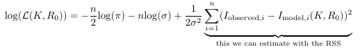
Using a Monte Carlo estimation. A formula to compute exactly the propagation of errors/variance in the data to the errors/variance in the estimates of the parameters is often very complex. The Hessian will only give us a lower bound (I personally find it more useful to see any potential strong correlation between parameters), and it is not so easy to implement. There is however a very blunt but effective way to get an idea of the propagation of errors and that is by performing a random simulation.
The full details of this method are explained in the covid.R file. Here we will show just the results of the simulation:
In this simulation, we simulated  times new data based on a true model with parameter values
  and
and  and with the variance of data points corresponding to the observed RSS of our fit. We also show in the right graph how the parameters
  and
and  are distributed for the same simulation. The parameters and are strongly correlated. This results in them having a large marginal/individual error, but the values
  and
and  have much less relative variation (this is why we changed the fitting parameters from and to and ).
Fitting by using the latest data and by using the analytical solution of the model
Now, we are almost at the end of this post, and we will make a new attempt to fit again the epidemiological curve, but now based on more new data.
What we do this time is make some small adaptations:
- The data is the number of total people that have gotten sick. This is different from the
 (infectious) and
  (recovered) output of the model. We make the comparison of the modelled
  with the data (the total that have gone sick).
 - In this comparison, we will use a scaling factor because the reported number of infected/infectious people is an underestimation of the true value, and this latter value is what the model computes. We use two scaling factors one for before and one for after February 12 (because at that time the definition for reporting cases had been changed).
- We make the population size a fitting variable. This will correct for the two assumptions that we have homogeneous mixing among the entire population of China and that
 of the population is susceptible. In addition, we make the infected people at the start a fitting variable. In this model, we will fit . There is data for a separate but it is not such an accurate variable (because the recovery and the infectious phase is not easy to define/measure/determine).
Because the computation of all these parameters is too difficult in a single optim function we solve the parameters separately in a nested way. In the most inner loop, we solve the scaling parameters (which can be done with a simple linear model), in the middle loop we solve the and with the optim function, in the outer loop we do a brute force search for the optimal starting point of  .
.
To obtain a starting condition we use a result from Harko, Lobo and Mak 2014 (Exact analytical solutions of the Susceptible-Infected-Recovered (SIR) epidemic model and of the SIR model with equal death and birth rates) who derived expressions for  , and in terms of a single differential equation. The equation below is based on their equations but expressed in slightly different terms:
![\[\frac{dS}{dt} = \beta (\frac{R(0)}{N}-1) \cdot S -\gamma \cdot S \, \text{log}(S/N) + \beta S^2/N\]](https://blog.ephorie.de/wp-content/ql-cache/quicklatex.com-378d5fdb6b0cb9161ebb494511f23729_l3.png "Rendered by QuickLaTeX.com")
We can solve this equation as a linear equation which gives us a good starting condition (small sidenote: using some form of differential equation is a general way of getting starting conditions, but the  might be noisy, in that case, one could integrate the expression).
The further details of the computation can be found in the covid.R script. Below you see a result of the outer loop where we did a brute force search (which gives an optimum around  for
for  ) and next to it a fitted curve for the parameters
  ,
,  ,
,  and
and  .
.
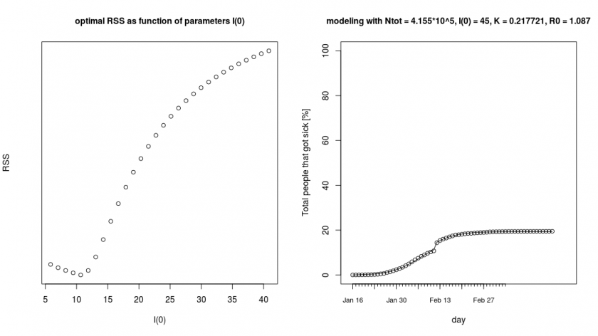
In this new fit, we get again a low reproduction number . One potential reason for this is that due to the measures that have been taken, the Chinese have been able to reduce the rate of the spread of the virus. The model is unaware of this and interprets this as a reduction that is due to immunity (decrease of susceptible people). However, only a very small fraction of the people have gained immunity (about  of the population got sick if we consider ). For the virus to stop spreading at already such a low fraction of sick people it must mean that the is very low.
Thus, an estimation of the parameters, based on this type of data, is difficult. When we see a decrease in the growth rate then one or more of the following four effects play a role: (1) The number of susceptible people has decreased sufficiently to overcome the reproduction rate . This relative decrease in susceptible people happens faster when the total number of people is smaller. (2) Something has changed about the conditions, the reproduction rate is not constant in time. For instance, with respiratory infections, it is common that the transfer rates depend on weather and are higher during winter. (3) The measures that are being taken against the disease are taking effect. (4) The model is too simple with several assumptions that overestimate the effect of the initial growth rate. This growth rate is very high  per day, and we observe a doubling every three days. This means that the time between generations is very short, something that is not believed to be true. It may be likely that the increase in numbers is partially due to variable time delay in the occurrence of the symptoms as well as sampling bias.
For statisticians, it is difficult to estimate what causes the changes in the epidemic curves. We should need more detailed information in order to fill in the gaps which do not seem to go away by having just more data (and this coronavirus creates a lot of data, possibly too much). But as human beings under threat of a nasty disease, we can at least consider ourselves lucky that we have a lot of options how the disease can fade away. And we can be lucky that we see a seemingly/effective reproduction rate that is very low, and also only a fraction of the population is susceptible.
Wrap up
So now we have done all this nice mathematics and we can draw accurately a modelled curve through all our data points. But is this useful when we model the wrong data with the wrong model? The difference between statistics and mathematics is that statisticians need to look beyond the computations.
- We need to consider what the data actually represents, how is it sampled, whether there are biases and how strongly they are gonna influence our analysis. We should actually do this ideally before we start throwing computations at the data. Or such computations will at most be exploratory analysis, but they should not start to live their own life without the data.
- And we need to consider how good a representation our models are. We can make expressions based on the variance in the data, but the error is also determined by the bias in our models.
At the present time, COVID-19 is making an enormous impact on our lives, with an unclear effect for the future (we even do not know when the measures are gonna stop, end of April, end of May, maybe even June?). Only time will tell what the economic aftermath of this coronavirus is gonna be, and how much it’s impact will be for our health and quality of life. But one thing that we can assure ourself about is that the ominous view of an unlimited exponential growth (currently going around on social media) is not data-driven.
In this post, I have explained some mathematics about fitting. However, I would like to warn for the blunt use of these mathematical formula’s. Just because we use a mathematical model does not mean that our conclusions/predictions are trustworthy. We need to challenge the premises which are the underlying data and models. So in a next post, “Contagiousness of COVID-19 Part 2: Why the Result of Part 1 is Useless”, I hope to explain what sort of considerations about the data and the models one should take into account and make some connections with other cases where statistics went in a wrong direction.
The cumulative curve looks like a Gompertz curve. Can’t it be modelled with nlm or gam ?
I am afraid that for the SIR model we have to do with the implicit differential equation (the one from Harko et. al who expressed the coupled ODE as a single ODE). I doubt that we can make an explicit function for y.
(I actually have to check again whether I did not make a mistake there, I might have made an error with a minus sign).
But different models might be good approximations. There are several that have used a logistic function.
Prof:
Excellent post.
Is it possible to use genetic algorithm to find optimum values of the parameters?
Definitely, have a look at the following paper (pp. 11): On some extensions to GA package: hybrid optimisation, parallelisation and islands evolution.
Bonjour. Pourrai-je savoir comment fixe-t-on les valeur de
par(),lower()etupper()dans la fonctionoptims’il vous plait?Hello! I don’t understand how to fix the value in
par(),lower()andupper(). Can we help with some explanations please?Well done. Amazing analysis …..Thank you.
What does R and D in the code represent ? ( Guess Recovered and Death!). I use for Infected the accumulative value i.e. (infected= cumsum(confirmed cases)- ( cumsum(recovered)-cumsum(death) ).
It would be such a great help if you make the graph to be plotted with auto date or even based on the data in the graphs. For example what if the data reflects until today , some graphs you have reflects until Feb 6. I know this might be straightforward for me to change it based on my case. But, it just a suggestion.
Hello Sal,
you are right about R and D
R = number of Recovered people
D = number of Diseased/Death people
I = *currently* Infected people
S = number of Susceptible people
You get indeed the number of currently infected cases by applying the formula:
currently infected cases = cumsum(confirmed cases)- ( cumsum(recovered)-cumsum(death)
However, in many reports the number of Recovered are not so accurate. (the number of Death is not so difficult to measure, and it might actually be even easier when you use statistics from like the differences in crude death rates).
So because the number of Recovered is not so accurate I chose for the final case to not model the I, but instead the I+R (or I+R+D, if you split R into death and recovered).
I+R+D = currently infected cases + cumsum(recovered)+ cumsum(death) = cumsum(confirmed cases)
If you model the ‘cumsum(confirmed cases)’, then you have less problems with the low accuracy in the number of recovered cases.
———————-
Regarding the adjustments to plotting of graphs. You are right that this could have been done better, and more general. I am often hard coding these things (but I do normally not use dates on the x-axis so I don’t get into much problems).
Should we maybe turn the code into a package on github where we can keep updating the code with such improvements?
I think it is an excellent idea to turn the code into a package! I would add the link in the main post above.