Logistic Regression as the Smallest Possible Neural Network

We already covered Neural Networks and Logistic Regression in this blog.

If you want to gain an even deeper understanding of the fascinating connection between those two popular machine learning techniques read on!

Let us recap what an artificial neuron looks like:

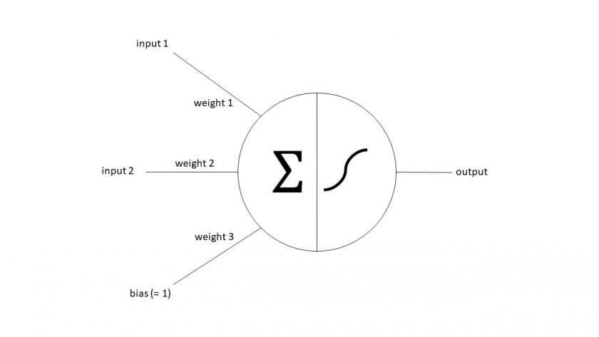
Mathematically it is some kind of non-linear activation function of the scalar product of the input vector and the weight vector. One of the inputs the so-called bias (neuron), is fixed at 1.

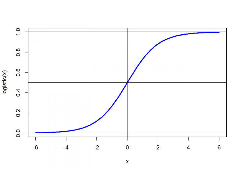
The activation function can e.g. be (and often is) the logistic function (which is an example of a sigmoid function):

logistic <- function(x) 1 / (1 + exp(-x))
curve(logistic, -6, 6, lwd = 3, col = "blue")
abline(h = c(0, 0.5, 1), v = 0)

Written mathematically an artificial neuron performs the following function:

   

Written this way that is nothing else but a logistic regression as a Generalized Linear Model (GLM) (which is basically itself nothing else but the logistic function of a simple linear regression)! More precisely it is the probability given by a binary logistic regression that the actual class is equal to 1. So, basically:

neuron = logistic regression = logistic(linear regression)

The following table translates the terms used in each domain:

Neural network	Logistic regression
Activation function	Link function
Weights	Coefficients
Bias	Intercept
Learning	Fitting

Interestingly enough, there is also no closed-form solution for logistic regression, so the fitting is also done via a numeric optimization algorithm like gradient descent (for some more mathematical details please consult my question on Stats.SE: How to specify logistic regression as transformed linear regression?). Gradient descent is also widely used for the training of neural networks (if you want to understand how it works see here: Why Gradient Descent Works (and How To Animate 3D-Functions in R)).

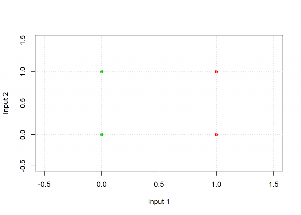
To illustrate this connection in practice we will again take the example from “Understanding the Magic of Neural Networks” to classify points in a plane, but this time with the logistic function and some more learning cycles. Have a look at the following table:

Input 1	Input 2	Output
1	0	0
0	0	1
1	1	0
0	1	1

If you plot those points with the colour coded pattern you get the following picture:

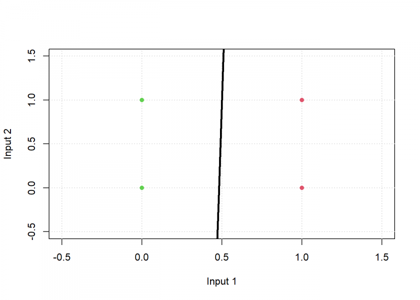
The task for the neuron is to find a separating line and thereby classify the two groups. Have a look at the following code:

# inspired by Kubat: An Introduction to Machine Learning, p. 72
plot_line <- function(w, col = "blue", add = "FALSE", type = "l")
  curve(-w[1] / w[2] * x - w[3] / w[2], xlim = c(-0.5, 1.5), ylim = c(-0.5, 1.5), col = col, lwd = 3, xlab = "Input 1", ylab = "Input 2", add = add, type = type)
neuron <- function(input) as.vector(logistic(input %*% weights)) # logistic function on scalar product of weights and input
eta <- 0.7 # learning rate

# examples
input <- matrix(c(1, 0,
                  0, 0,
                  1, 1,
                  0, 1), ncol = 2, byrow = TRUE)
input <- cbind(input, 1) # bias for intercept of line
output <- c(0, 1, 0, 1)
weights <- rep(0.2, 3) # random initial weights

plot_line(weights, type = "n"); grid()
points(input[ , 1:2], pch = 16, col = (output + 2))

# training of weights of neuron
for (i in 1:1e5) {
  for (example in 1:length(output)) {
    weights <- weights + eta * (output[example] - neuron(input[example, ])) * input[example, ]
  }
}
plot_line(weights, add = TRUE, col = "black")

# test: applying neuron on input
round(apply(input, 1, neuron))
## [1] 0 1 0 1

As you can see, the result matches the desired output, graphically the black line separates the green from the red points: the neuron has learned this simple classification task. Now let us do the same with logistic regression:

# logistic regression - glm stands for generalized linear model
logreg <- glm(output ~ ., data = data.frame(input, output), family = binomial) 

# test: prediction logreg on input
round(predict(logreg, data.frame(input), "response"), 3)
## Warning in predict.lm(object, newdata, se.fit, scale = 1, type = if (type == :
## prediction from a rank-deficient fit may be misleading
## 1 2 3 4 
## 0 1 0 1

plot_line(weights, type = "n"); grid()
points(input[ , 1:2], pch = 16, col = (output + 2))
plot_line(weights, add = TRUE, col = "darkgrey")
plot_line(coef(logreg)[c(2:3, 1)], add = TRUE, col = "black")

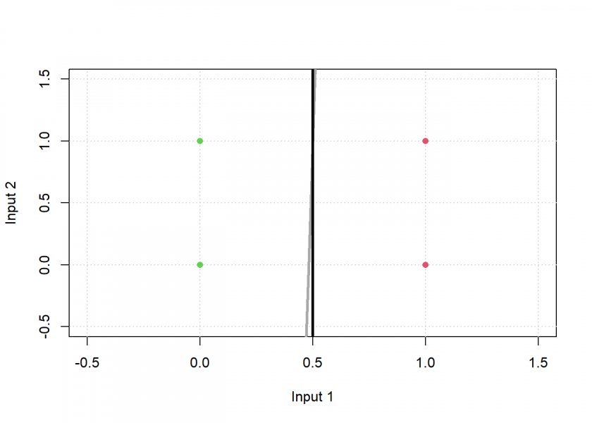
Here we used the same plotting function with the coefficients of the logistic regression (instead of the weights of the neuron) as input: as you can see the black line perfectly separates both groups, even a little bit better than the neuron (in dark grey). Fiddling with the initialization, the learning rate, and the number of learning cycles should move the neuron’s line even further towards the logistic regression’s perfect solution.

I always find it fascinating to understand the hidden connections between different realms and I think this insight is especially cool: logistic regression really is the smallest possible neural network!