Why Gradient Descent Works (and How To Animate 3D-Functions in R)

The workhorse of Machine Learning is Gradient Descent. If you want to understand how and why it works and, along the way, want to learn how to plot and animate 3D-functions in R read on!

Gradient Descent is a mathematical algorithm to optimize functions, i.e. finding their minima or maxima. In Machine Learning it is used to minimize the cost function of many learning algorithms, e.g. artificial neural networks a.k.a. deep learning. The cost function simply is the function that measures how good a set of predictions is compared to the actual values (e.g. in regression problems).

The gradient (technically the negative gradient) is the direction of steepest descent. Just imagine a skier standing on top of a hill: the direction which points into the direction of steepest descent is the gradient!

Mathematically the gradient “stores” all the partial derivative information of a multivariable function, basically the slopes with respect to the directions of all axes. So, the Gradient Descent-algorithm always moves in the direction of the gradient to reach the minimum of the function (NB: in some cases unfortunately only a local minimum!), like our skier always taking the steepest route to reach the valley as fast as possible!

The question is: why does a bundle of partial derivatives point in the direction of the steepest descent? I answered this question some time ago here: Math.SE: Why is gradient the direction of steepest ascent?

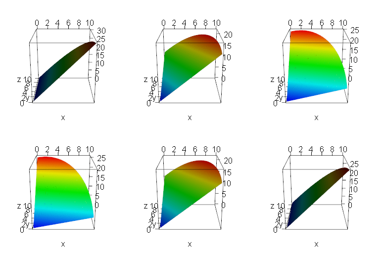
To give some intuition why the gradient (technically the negative gradient) has to point in the direction of steepest descent I created the following animation.

It shows all of the points that can be reached by a vector of a given length and two variables x and y that are multiplied by a constant and summed up to give a very simple linear function (which give very simple directional derivatives).

I then vary the constants relative to each other: when the constant of x goes up (down) the constant of y goes down (up). The red area equals the highest point which means that you have the steepest descent from there.

As can be seen, this point varies smoothly with the proportion of the constants which represent the derivatives in each direction!

Only when one constant equals zero do we have a corner solution, when both constants are the same the red area is exactly in the middle. There is no good reason why the red area (= steepest descent) should jump around between those points.

This means that the gradient will always point in the direction of the steepest descent (nb: which is of course not a proof but a hand-waving indication of its behaviour to give some intuition only!)

I created the animation with the rgl package (on CRAN) and ImageMagick (see aso this post: Creating a Movie with Data from Outer Space in R).

The following fully documented code can be taken as a template to create plots and animations of 3D-functions with constraints (or inequalities). f is defined as follows:

where is varied between and .

library(rgl)
# create many x and y pairs as input of function
x <- y <- seq(0, 10, 0.01)

# define 3D-function with constraint
f <- function(x, y) {
  ifelse(sqrt(x^2 + y^2) < 10, (3-n)*x + n*y, NA)
}

# for rainbow colouring the function
nbcol <- 100
color <- rev(rainbow(nbcol, start = 0/6, end = 4/6))
zcol  <- cut(z, nbcol)

# loop for 3D-plots of function with n from 0 to 3 and back
olddir <- setwd("anim") # change path accordingly
nlim <- 3
step <- 0.1
niter <- c(seq(0, nlim, step), seq(nlim-step, step, -step))
for (i in 1:length(niter)) {
  n <- niter[i]
  z <- outer(x, y, f)
  zcol <- cut(z, nbcol)
  persp3d(x, y, z, col = color[zcol])
  filename <- paste0("pic", ifelse((i-1) < 10, paste0("0", (i-1)), (i-1)), ".png")
  rgl.snapshot(filename, fmt = "png", top = TRUE)
}

# make animated gif with ImageMagick
system("cmd.exe", input = "convert -delay 20 -loop 0 pic*.png gradient.gif")
setwd(olddir)

I am always fascinated by how versatile R is!