

R is one of the best choices when it comes to quantitative finance. Here we will show you how to load financial data, plot charts and give you a step-by-step template to backtest trading strategies. So, read on…
We begin by just plotting a chart of the Standard & Poor’s 500 (S&P 500), an index of the 500 biggest companies in the US. To get the index data and plot the chart we use the powerful quantmod package (on CRAN). After that we add two popular indicators, the simple moving average (SMI) and the exponential moving average (EMA).
Have a look at the code:
library(quantmod)
## Loading required package: xts
## Loading required package: zoo
##
## Attaching package: 'zoo'
## The following objects are masked from 'package:base':
##
##     as.Date, as.Date.numeric
## Loading required package: TTR
## Version 0.4-0 included new data defaults. See ?getSymbols.

getSymbols("^GSPC", from = "2000-01-01")
## 'getSymbols' currently uses auto.assign=TRUE by default, but will
## use auto.assign=FALSE in 0.5-0. You will still be able to use
## 'loadSymbols' to automatically load data. getOption("getSymbols.env")
## and getOption("getSymbols.auto.assign") will still be checked for
## alternate defaults.
##
## This message is shown once per session and may be disabled by setting
## options("getSymbols.warning4.0"=FALSE). See ?getSymbols for details.
## [1] "^GSPC"

head(GSPC)
##            GSPC.Open GSPC.High GSPC.Low GSPC.Close GSPC.Volume
## 2000-01-03   1469.25   1478.00  1438.36    1455.22   931800000
## 2000-01-04   1455.22   1455.22  1397.43    1399.42  1009000000
## 2000-01-05   1399.42   1413.27  1377.68    1402.11  1085500000
## 2000-01-06   1402.11   1411.90  1392.10    1403.45  1092300000
## 2000-01-07   1403.45   1441.47  1400.73    1441.47  1225200000
## 2000-01-10   1441.47   1464.36  1441.47    1457.60  1064800000
##            GSPC.Adjusted
## 2000-01-03       1455.22
## 2000-01-04       1399.42
## 2000-01-05       1402.11
## 2000-01-06       1403.45
## 2000-01-07       1441.47
## 2000-01-10       1457.60

tail(GSPC)
##            GSPC.Open GSPC.High GSPC.Low GSPC.Close GSPC.Volume
## 2019-04-24   2934.00   2936.83  2926.05    2927.25  3448960000
## 2019-04-25   2928.99   2933.10  2912.84    2926.17  3425280000
## 2019-04-26   2925.81   2939.88  2917.56    2939.88  3248500000
## 2019-04-29   2940.58   2949.52  2939.35    2943.03  3118780000
## 2019-04-30   2937.14   2948.22  2924.11    2945.83  3919330000
## 2019-05-01   2952.33   2954.13  2923.36    2923.73  3645850000
##            GSPC.Adjusted
## 2019-04-24       2927.25
## 2019-04-25       2926.17
## 2019-04-26       2939.88
## 2019-04-29       2943.03
## 2019-04-30       2945.83
## 2019-05-01       2923.73

chartSeries(GSPC, theme = chartTheme("white"), subset = "last 10 months", show.grid = TRUE)
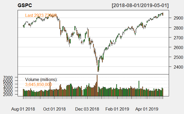
addSMA(20)
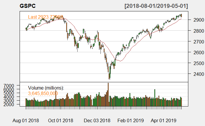
addEMA(20)

As you can see the moving averages are basically smoothed out versions of the original data shifted by the given number of days. While with the SMA (red curve) all days are weighted equally with the EMA (blue curve) the more recent days are weighted stronger, so that the resulting indicator detects changes quicker. The idea is that by using those indicators investors might be able to detect longer-term trends and act accordingly. For example, a trading rule could be to buy the index whenever it crosses the MA from below and sell when it goes the other direction. Judge for yourself if this could have worked.
Well, having said that it might not be that easy to find out the profitability of certain trading rules just by staring at a chart. We are looking for something more systematic! We would need a decent backtest! This can of course also be done with R, an excellent choice is the PerformanceAnalytics package (on CRAN).
To backtest a trading strategy I provide you with a step-by-step template:
- Load libraries and data
- Create your indicator
- Use indicator to create equity curve
- Evaluate strategy performance
As an example, we want to test the idea that it might be profitable to sell the index when the financial markets exhibit significant stress. Interestingly enough “stress” can be measured by certain indicators that are freely available. One of them is the National Financial Conditions Index (NFCI) of the Federal Reserve Bank of Chicago (https://www.chicagofed.org/publications/nfci/index):
The Chicago Fed’s National Financial Conditions Index (NFCI) provides a comprehensive weekly update on U.S. financial conditions in money markets, debt and equity markets and the traditional and “shadow” banking systems. […] The NFCI [is] constructed to have an average value of zero and a standard deviation of one over a sample period extending back to 1971. Positive values of the NFCI have been historically associated with tighter-than-average financial conditions, while negative values have been historically associated with looser-than-average financial conditions.
To make it more concrete we want to create a buy signal when the index is above one standard deviation in negative territory and a sell signal otherwise.
Have a look at the following code:
# Step 1: Load libraries and data
library(quantmod)
library(PerformanceAnalytics)

getSymbols('NFCI', src = 'FRED', , from = '2000-01-01')
## [1] "NFCI"

NFCI <- na.omit(lag(NFCI)) # we can only act on the signal after release, i.e. the next day
getSymbols("^GSPC", from = '2000-01-01')
## [1] "GSPC"

data <- na.omit(merge(NFCI, GSPC)) # merge data
data$GSPC <- ROC(Cl(data), type = "discrete") # calculate returns of closing prices
data <- na.omit(data)

# Step 2: Create your indicator
data$sig <- ifelse(data$NFCI < 1, 1, 0)
data$sig <- na.locf(data$sig)

# Step 3: Use indicator to create equity curve
perf <- na.omit(merge(data$sig * data$GSPC, data$GSPC))
colnames(perf) <- c("Stress-based strategy", "SP500")

# Step 4: Evaluate strategy performance
table.DownsideRisk(perf)
##                                            Stress-based strategy   SP500
## Semi Deviation                                            0.0169  0.0187
## Gain Deviation                                            0.0155  0.0169
## Loss Deviation                                            0.0175  0.0197
## Downside Deviation (MAR=43.3333333333333%)                0.0205  0.0223
## Downside Deviation (Rf=0%)                                0.0162  0.0180
## Downside Deviation (0%)                                   0.0162  0.0180
## Maximum Drawdown                                          0.4759  0.5624
## Historical VaR (95%)                                     -0.0375 -0.0401
## Historical ES (95%)                                      -0.0536 -0.0599
## Modified VaR (95%)                                       -0.0358 -0.0401
## Modified ES (95%)                                        -0.0626 -0.0758

table.Stats(perf)
##                 Stress-based strategy     SP500
## Observations                1229.0000 1229.0000
## NAs                            0.0000    0.0000
## Minimum                       -0.1498   -0.1820
## Quartile 1                    -0.0100   -0.0110
## Median                         0.0019    0.0024
## Arithmetic Mean                0.0015    0.0014
## Geometric Mean                 0.0013    0.0010
## Quartile 3                     0.0141    0.0146
## Maximum                        0.1551    0.1551
## SE Mean                        0.0007    0.0007
## LCL Mean (0.95)                0.0002   -0.0001
## UCL Mean (0.95)                0.0028    0.0028
## Variance                       0.0005    0.0006
## Stdev                          0.0232    0.0255
## Skewness                      -0.2415   -0.3893
## Kurtosis                       5.0481    6.1402

charts.PerformanceSummary(perf)

chart.RelativePerformance(perf[ , 1], perf[ , 2])

chart.RiskReturnScatter(perf)

The first chart shows that the stress-based strategy (black curve) clearly outperformed its benchmark, the S&P 500 (red curve). This can also be seen in the second chart, showing the relative performance. In the third chart, we see that both return (more) and (!) risk (less) of our backtested strategy are more favourable compared to the benchmark.
So, overall, this seems to be a viable strategy! But of course, before investing real money many more tests have to be performed! You can use this framework for backtesting your own ideas.
Here is not the place to explain all of the above tables and plots but as you can see both packages are immensely powerful, and I have only shown you a small fraction of their capabilities. To use their full potential, you should have a look at the extensive documentation that comes with it on CRAN.
DISCLAIMER
This post is written on an “as is” basis for educational purposes only, can contain errors, and comes without any warranty. The findings and interpretations are exclusively those of the author and are not endorsed by or affiliated with any third party.
This post provides no investment advice! No responsibility is taken whatsoever if you lose money.
(If you make any money though I would be happy if you would buy me a coffee… that is not too much to ask, is it? 😉 )
UPDATE April 14, 2021
If you want to learn how to backtest options strategies, see my post here: Backtesting Options Strategies with R.
UPDATE October 9, 2021
I created a video for this post (in German):
UPDATE April 10, 2023
I updated the backtest to the current date. I also changed the calculation of the returns to type = "discrete" because PerformanceAnalytics seems to expect simple returns, i.e. geometric chaining (see the answer from the developer of the quantmod package here).
UPDATE May 30, 2024
I updated the backtest to the current date. I also corrected some inconsistencies in the handling of NAs.
Do you have the code In Python?
No and I would guess that R is better suited than Python to perform this kind of analysis. Why don’t you try it out in R, with this template it should be easy enough!
Dear Thomas: I have published a post where you can learn R the easy way:
Learning R: The Ultimate Introduction (incl. Machine Learning!)
Hope that helps!
Hi,
I got a few different meanings. It is not clear why if else(data$NFS I < 1, 1, 0). Codes here https://github.com/VladPerervenko/GSPC
What do you mean by “meanings”? What did you get? Perhaps because of different end dates?
Translation errors. Mean difference in the data tables. Thanks for the article.
Ok, I didn’t run your code but how many observations do you have? Is it the same number I have? My last observation is 2019-05-01.
I have the latest date 2019-05-21. This is the reason for the difference. Good luck
Your strategy outperforms for like 1 hour and does nothing the rest of the time. Effectively you have a sample size of one. It is not to be trusted really. I would edit the conclusions quite heavily.
Thank you, Nick, I am well aware of that. I am just presenting the framework here for your own experiments – I do not give any investment advice or any superior trading strategies.
Hi,
Thanks for this! What’s still unclear to me is how you action the buy/sell signals. If I do
table(data$sig)I see 5209 1s and only 164 0s. So if it’s 1 you buy? But if you sell so infrequently, this means that you need to continue putting money and money into it, isn’t it? From investment videos I’ve watched It seems like a buy signal has a take-profit of x above where you sell (and then a stop-loss but let’s not even get into that). So I would imagine transactions would look like 1 0 1 0 1 0 0 1 0 1 1 0 something like this… but is that not what this trading strategy is doing? Sorry if I’m dense!Thank you for your question, Amit.
It means that you should be in the market when the indicator says 1 and out of the market when it says 0., so basically a buy signal is the change from o to 1, and a sell signal the change from 1 to 0 respectively.
Hope this clarifies things.
Hi
I’m getting this error:
when running the:
charts.PerformanceSummary(perf)Any ideas why?
Hi Tomer,
I just reran the code and I am sorry, but I cannot reproduce the error. Everything seems fine.
Interesting approach with R. For retail traders who don’t code, visual backtesting tools are starting to fill this gap. You define your strategy with drag-and-drop blocks and the platform handles the execution logic.
The tricky part with any backtesting approach is making sure you’re not using future data. Most Pine Script community indicators use close (current bar) instead of close[1] (confirmed bar), which makes backtests look better than they should. Tools that enforce close[1] at the engine level solve this problem by design.