
 It is such a beautiful day outside, lot’s of sunshine, spring at last… and we are now basically all grounded and sitting here, waiting to get sick.
So, why not a post from the new epicentre of the global COVID-19 pandemic, Central Europe, more exactly where I live: Germany?! Indeed, if you want to find out what the numbers tell us how things might develop here, read on!
We will use the same model we already used in this post: Epidemiology: How contagious is Novel Coronavirus (2019-nCoV)?. You can find all the details there and in the comments.
library(deSolve)

# https://en.wikipedia.org/wiki/2020_coronavirus_pandemic_in_Germany#Statistics
Infected <- c(16, 18, 21, 26, 53, 66, 117, 150, 188, 240, 349, 534, 684, 847, 1110, 1458, 1881, 2364, 3057, 3787, 4826, 5999)
Day <- 1:(length(Infected))
N <- 83149300 # population of Germany acc. to Destatis

old <- par(mfrow = c(1, 2))
plot(Day, Infected, type ="b")
plot(Day, Infected, log = "y")
abline(lm(log10(Infected) ~ Day))
title("Total infections COVID-19 Germany", outer = TRUE, line = -2)
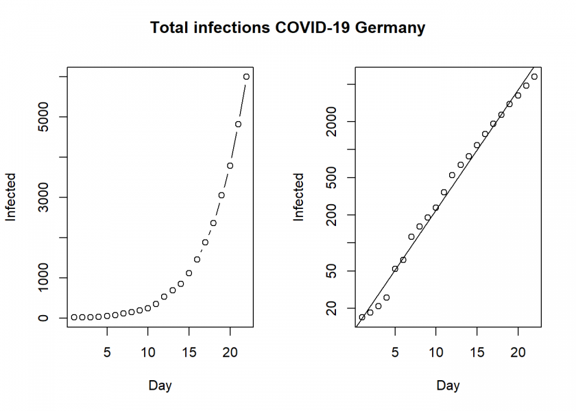
This clearly shows that we have an exponential development here, unfortunately as expected.
SIR <- function(time, state, parameters) {
par <- as.list(c(state, parameters))
with(par, {
dS <- -beta/N * I * S
dI <- beta/N * I * S - gamma * I
dR <- gamma * I
list(c(dS, dI, dR))
})
}
init <- c(S = N-Infected[1], I = Infected[1], R = 0)
RSS <- function(parameters) {
names(parameters) <- c("beta", "gamma")
out <- ode(y = init, times = Day, func = SIR, parms = parameters)
fit <- out[ , 3]
sum((Infected - fit)^2)
}
Opt <- optim(c(0.5, 0.5), RSS, method = "L-BFGS-B", lower = c(0, 0), upper = c(1, 1)) # optimize with some sensible conditions
Opt$message
## [1] "CONVERGENCE: REL_REDUCTION_OF_F <= FACTR*EPSMCH"
Opt_par <- setNames(Opt$par, c("beta", "gamma"))
Opt_par
## beta gamma
## 0.6427585 0.3572415
t <- 1:80 # time in days
fit <- data.frame(ode(y = init, times = t, func = SIR, parms = Opt_par))
col <- 1:3 # colour
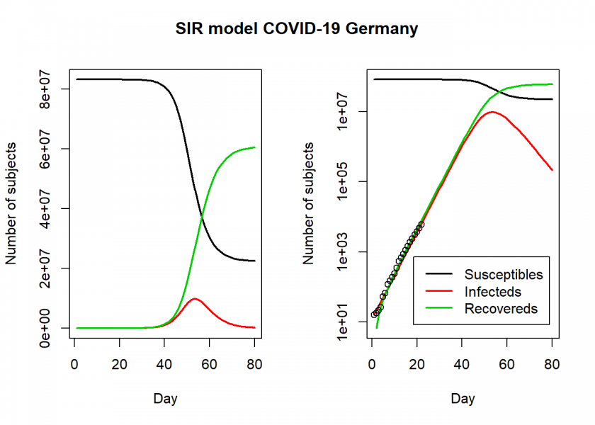
matplot(fit$time, fit[ , 2:4], type = "l", xlab = "Day", ylab = "Number of subjects", lwd = 2, lty = 1, col = col)
matplot(fit$time, fit[ , 2:4], type = "l", xlab = "Day", ylab = "Number of subjects", lwd = 2, lty = 1, col = col, log = "y")
## Warning in xy.coords(x, y, xlabel, ylabel, log = log): 1 y value <= 0
## omitted from logarithmic plot
points(Day, Infected)
legend("bottomright", c("Susceptibles", "Infecteds", "Recovereds"), lty = 1, lwd = 2, col = col, inset = 0.05)
title("SIR model COVID-19 Germany", outer = TRUE, line = -2)
par(old)

R0 <- setNames(Opt_par["beta"] / Opt_par["gamma"], "R0")
R0
##       R0
## 1.799227

fit[fit$I == max(fit$I), "I", drop = FALSE] # height of pandemic
##          I
## 54 9765121

max_infected <- max(fit$I)
max_infected / 5 # severe cases
## [1] 1953024

max_infected * 0.06 # cases with need for intensive care
## [1] 585907.3

# https://www.newscientist.com/article/mg24532733-700-why-is-it-so-hard-to-calculate-how-many-people-will-die-from-covid-19/
max_infected * 0.007 # deaths with supposed 0.7% fatality rate
## [1] 68355.85
So, according to this model, the height of the pandemic will be reached by the end of April, beginning of May. About 10 million people would be infected by then, which translates to about 2 million severe cases, about 600,000 cases in need of intensive care (there are about 28,000 ICU beds in Germany with an average utilization rate of around 80%) and up to 70,000 deaths.
Those are the numbers our model produces and nobody knows whether they are correct while everybody hopes they are not. One thing has to be kept in mind though: the numbers used in the model are from before the shutdown (for details see here: DER SPIEGEL: Germany Moves To Shut Down Most of Public Life). So hopefully those measures will prove effective and the actual numbers will turn out to be much, much lower.
I wish you all the best and stay healthy!
UPDATE March 17, 2020
The German National Institute for Public Health “Robert Koch Institute” (RKI) just announced that there could be up to 10 million infections in the next few months. This agrees with my model above.
Also, the current number of confirmed infections (about 8,200 cases) is within a small error margin (about 3%) what my model predicted for today.
Source: DER SPIEGEL: Coronavirus Could Infect Up to 10 Million in Germany
UPDATE February 23, 2021
Today we nearly reached the number of deaths I predicted about a year ago.
It can be argued that the prediction was pretty accurate considering the “flatten-the-curve”-measures that didn’t prevent the deaths but simply spread them out to prevent overloading the healthcare system. Additionally, the calculation was based on the original virus, with the new mutations we face a completely new situation.
I have never been more saddened by one of my predictions come true. It is a triumph for mathematics and statistics but a horrible tragedy for humanity.
Stay healthy and keep up the morale, there is light at the end of the tunnel: COVID-19 vaccine “95% effective”: It doesn’t mean what you think it means!
Hi,
I’m trying to understand your model. What I can’t wrap my head around is how you estimate the recovereds, as they are not part of your inputs: As I understand it, the number of infected is total infected, not active infected, so I’m not sure how you identify gamma.
Best, Owe
To understand the model better you can find out more here: https://blog.ephorie.de/epidemiology-how-contagious-is-novel-coronavirus-2019-ncov.
Basically, the three differential equations provide some sort of rigid frame: by doing the optimization you kind of cascade through them simultaneously so that all parameters are tuned at once. Because the equations are all connected by the different parameters you automatically get fitting values for all of them, some of them indirectly! Hope this helps
Owe,
the R-compartment of the SIR model should instead be named ‘removed’. It does not mean that people there have actually recovered from illness. It just means they move to a state where they can’t infect susceptibles any more – they could still be ill, home quarantined, in hospital, intensive care or even dead.
@Learning Machines
Shouldn’t the fit be on (daily) incidence instead of on cumulative infected? It doesn’t make much of a difference probably because in the exponential spreading phase the integral of an exponential curve remains an exponential curve. But uncertainties and trend changes are more easy to spot when using incidence data – that is (diff(infected).
https://ibb.co/VCBQ7fG
FYI: The underlying data file is https://interaktiv.morgenpost.de/corona-virus-karte-infektionen-deutschland-weltweit/data/Coronavirus.history.v2.csv
What would be needed are the currently infected persons (cumulative infected minus the removed, i.e. recovered or dead), but I couldn’t find the numbers of recovered persons and the difference isn’t that big anyway at the moment because we are still in the relatively early stages (i.e. only a few recoveries).
On top of that, the error margins of all numbers that are available and of the fitted parameters of the model are way bigger than those small differences.
When you look at the model you provided a link to you will see that they arrive at very similar projections.
Hi Wolfgang,
it seems that the source https://interaktiv.morgenpost.de/corona-virus-karte-infektionen-deutschland-weltweit/data/Coronavirus.history.v2.csv is not maintained any more. Until yesterday it was updated every night, but that has stopped. Do you happen to know if there is a new file available, and if so: can you share the file name ?
thanks
Reinhard
Considering the importance of the topic, I am surprised by this modelling that I first saw on R-Bloggers (sadly the comments are turned off there). There are a few very key issues:
– The use of observations: why use the death rate of Korea when the “modelling” uses data for Germany? The current fatality rate in Germany is 0.2%, not 0.7%. In addition, where are the 20% severe cases and 6% intensive care coming from?
– The treatment of uncertainty: there is none. All the modelling is based on the above data, which are by themselves very uncertain. The model has to consider these uncertainties.
– Why does the model integrate data only until March 15th while the piece was published March 17th and the latest data to update the modelling?
There are a number of – scientific – peer-reviewed articles that were recently published on the spread, R0, etc. I am therefore surprised there is no reference to any of these in your blog.
A disclaimer on the hypothetical and uncertain nature of the results, highlighting the issue with such modelling would be very welcome – particularly on the R-Bloggers which could have more audience than this blog.
Thank you for your feedback! R-bloggers doesn’t allow comments in general but you would be surprised how popular my blog is.
Concerning your issues:
– The death rate in Germany is, fortunately, lower at the moment but every patient is getting the best intensive care possible… that is going to change as soon as the healthcare system gets overwhelmed (what everybody is trying to prevent). Another effect is that we are in a relatively early phase, for many the fight has just begun… and many will, unfortunately, lose it. The other numbers are from the outbreak in China.
– I agree that there are big uncertainties. As I wrote in the article please consult Epidemiology: How contagious is Novel Coronavirus (2019-nCoV)? and the comments there.
– I published the article in the morning of March 17 with the then-available data and added an update later the same day.
Hope this clarifies your concerns
Popular and correct are two different things in when it comes to science.
This piece could help put your modelling into perspective: https://static1.squarespace.com/static/5b68a4e4a2772c2a206180a1/t/5e70eb32b16229792eb14836/1584458547530/ReviewOfFergusson.pdf
“Popular and correct are two different things in [sic!] when it comes to science.” Wow, now you are trying to teach me how science works? This was addressing your point of “more audience than this blog” and the possibility of comments on R-bloggers, and you know that. Seems like a cheap try to discredit my research. Please be careful with such polemic statements.
Anyway, thank you for the link: it might be helpful if you could provide some management abstract of the paper (i.e. why you posted it)… Thank you again.
Thanks for doing this. Very useful. I tried your algorithm on some other countries and the results were a bit mixed. The Ro ranged between 1.2 to 2.9 and it’s corresponding impact of infecting % of population. Would you mind going over my working to see if there are any issues.
Thanks in advance.
Kind regards
Joe
Thank you for your feedback. If you post your code here I would have a look.
Thanks for that.
– I have uploaded code to github:
https://github.com/JoeFernando/corona
* Please run the analysis.r script to generate the forecast
* I have saved the last forecast I did in the output directory
* The output for Germany closely matches your numbers, some 10mil infections
* These are my questions:
1. Why do some countries have a high Ro and a corresponding pct infection rate (see the df output from #Generate the forecast)
2. Problem countries – South Korea, Japan, Iran. Is the problem in forecast related to data quality or do we need to tune model parameters?
3. The model shows that by Jun20 the infection will largely die out…..is that correct?
Really appreciate you taking the time to help us out.
Thanks once again.
Kind regards
Joe
Thank you for your work!
Concerning your questions:
1. The main problem is, in my opinion, the reported number of cases. In many countries, there are just so many more cases but not enough testing.
2. Could really be both!
3. Well, for example in Germany it would if left unabated. But without flattening the curve we would have apocalyptic scenes. Flattening the curve tries to avoid a total collapse of the system but it prolongs the problem in a way.
Thanks for educating all of us. This has been an eye-opening exercise.
Here, in Sydney, Australia a lot of decision makers are living under a rock with hope as the only solution.
Your model has had a lot of practical value to me, so thank you for taking the time and effort.
Stay safe.
Thanks once again.
Kind regards
Joe
Dear Joe: Thank you so much for your great feedback!
I think in general all decision-makers around the world are only gradually waking up to this new reality. It has been (and still is) an exercise with a steep learning curve and a lesson in humility for all of us.
Stay healthy and all the best to Down Under from Germany
h
Could we take the data file https://interaktiv.morgenpost.de/corona-virus-karte-infektionen-deutschland-weltweit/data/Coronavirus.history.v2.csv and run your model with currently infected persons (cumulative infected minus the removed, i.e. recovered or dead) to obtain a better estimation? Thanks
Well, perhaps you want to give it a try and post your results here? I think the problem is that it is not clear where the “recovered” come from because there is no obligation to report those cases in Germany (unfortunately).
This is my code for the case of Spain and the results are also included at the end following your format. Any feedback is welcome
library(deSolve) # read data coronavirus <- read.csv("Coronavirus.history.v2.csv") head(coronavirus) table(coronavirus$label) coronaspain <- subset(coronavirus, label == "Spanien") head(coronaspain) tail(coronaspain) coronaspain$netconfirmed <- coronaspain$confirmed - coronaspain$recovered - coronaspain$deaths coronaspain$day <- 1:(length(coronaspain$netconfirmed)) N <- 47650000 # population of Spain, wikipedia, de iure old = 10 coronaspain10 = 10) head(coronaspain10) coronaspain10$day <- 1:(length(coronaspain10$netconfirmed)) old <- par(mfrow = c(1, 2)) plot(confirmed ~ day, data = coronaspain10, type ="b") plot(confirmed ~ day, data = coronaspain10, log = "y") abline(lm(log10(confirmed) ~ day, data = coronaspain10)) title("Total infections COVID-19 Spain", outer = TRUE, line = -2) SIR <- function(time, state, parameters) { par <- as.list(c(state, parameters)) with(par, { dS <- -beta/N * I * S dI <- beta/N * I * S - gamma * I dR <- gamma * I list(c(dS, dI, dR)) }) } init <- c(S = N-coronaspain10$netconfirmed[1], I = coronaspain10$netconfirmed[1], R = 0) RSS <- function(parameters) { names(parameters) <- c("beta", "gamma") out <- ode(y = init, times = coronaspain10$day, func = SIR, parms = parameters) fit <- out[ , 3] sum((coronaspain10$netconfirmed - fit)^2) } Opt <- optim(c(0.5, 0.5), RSS, method = "L-BFGS-B", lower = c(0, 0), upper = c(1, 1)) # optimize with some sensible conditions Opt$message ## [1] "CONVERGENCE: REL_REDUCTION_OF_F <= FACTR*EPSMCH" Opt_par <- setNames(Opt$par, c("beta", "gamma")) Opt_par ## beta gamma ## 0.6708997 0.3291007 t <- 1:80 # time in days fit <- data.frame(ode(y = init, times = t, func = SIR, parms = Opt_par)) col <- 1:3 # colour matplot(fit$time, fit[ , 2:4], type = "l", xlab = "Day", ylab = "Number of subjects", lwd = 2, lty = 1, col = col) matplot(fit$time, fit[ , 2:4], type = "l", xlab = "Day", ylab = "Number of subjects", lwd = 2, lty = 1, col = col, log = "y") ## Warning in xy.coords(x, y, xlabel, ylabel, log = log): 1 y value <= 0 ## omitted from logarithmic plot points(coronaspain10$day, coronaspain10$netconfirmed) legend("bottom", cex= 0.6, bty = 'n', y.intersp = 0.3, c("Susceptibles", "Confirm - Recov - deads", "Recovereds"), lty = 1, lwd = 2, col = col, inset = 0.05) title("SIR model COVID-19 Spain", outer = TRUE, line = -2) par(old) R0 <- setNames(Opt_par["beta"] / Opt_par["gamma"], "R0") R0 ## R0 ## 2.038585 fit[fit$I == max(fit$I), "I", drop = FALSE] # height of pandemic ## I ## 45 7598201 max_infected <- max(fit$I) max_infected / 5 # severe cases ## [1] 1519640 max_infected * 0.06 # cases with need for intensive care ## [1] 455892.1 # https://www.newscientist.com/article/mg24532733-700-why-is-it-so-hard-to-calculate-how-many-people-will-die-from-covid-19/ max_infected * 0.007 # deaths with supposed 0.7% fatality rate ## [1] 53187.41Thank you, where did you get
Coronavirus.history.v2.csv?The code looks fine to me.
Is this an error here :
coronaspain10 = 10)
Are removing “netconfirm” cases with value 0?
Wolfgang Flamme posted the link here yesterday 🙂
BTW, could you tell me if
coronaspain$netconfirmed <- coronaspain$confirmed – coronaspain$recovered – coronaspain$deaths
is the correct variable to introduce in the model? or should it be
coronaspain$netconfirmed <- coronaspain$confirmed – coronaspain$deaths
Thanks
I would think that the first definition is correct (it depends a little bit on the way the cases are recorded, i.e. whether “confirmed” is adjusted for deaths already, but I don’t think it is).
Ah, ok! Thank you 🙂
Thanks for such a great post on the COVID-19 models. I’ve also updated for the UK in a similar post here
https://tjwilding.wordpress.com/2020/03/20/epidemic-modelling-of-covid-19-in-the-uk-using-an-sir-model/
Please let me know if you think anything should be added and thanks again.
This is my code for the case of Bangladesh— I understand the zero values have impact on log-scale graph; but I also noticed that the beta and gamma values are so close in this model which is 0.5045723 and 0.4954277 respectively that ultimately generates a meaningless SIR graph. Any thoughts?
require(tidyverse) require(deSolve) require(scales) Infected <- c(3, 0, 0, 0, 0, 0, 0, 2, 3, 2, 4, 3, 3, 5, 2, 6, 6) Day <- 1:(length(Infected)) N <- 171421675 # population of Bangladesh 171,421,675 old <- par(mfrow = c(1, 2)) plot(Day, Infected, type ="b") plot(Day, Infected, log = "y") abline(lm(log10(Infected) ~ Day)) title("Confirmed Cases 2019-nCoV Bangladesh", outer = TRUE, line = -2) data > SIR = S + I + R; paramter = beta, gamma; time = time # d/dt(S) = -beta*I*S/N; d/dt(I) = beta*I*S/N - gamma*I; d/dt(R) = gamma*I SIR <- function(time, state, parameters) { par <- as.list(c(state, parameters)) with(par, { dS <- -beta/N * I * S dI <- beta/N * I * S - gamma * I dR <- gamma * I list(c(dS, dI, dR)) }) } init <- c(S = N-Infected[1], I = Infected[1], R = 0) RSS <- function(parameters) { names(parameters) <- c("beta", "gamma") out <- ode(y = init, times = Day, func = SIR, parms = parameters) fit <- out[ , 3] sum((Infected - fit)^2) } Opt <- optim(c(0.5, 0.5), RSS, method = "L-BFGS-B", lower = c(0, 0), upper = c(1, 1)) # optimize with some sensible conditions Opt$message Opt_par <- setNames(Opt$par, c("beta", "gamma")) Opt_par t <- 1:70 # time in days fit <- data.frame(ode(y = init, times = t, func = SIR, parms = Opt_par)) ggplot(fit,aes(x = time))+ geom_line(aes(y=S,colour="Susceptible"), size = 1) + geom_line(aes(y=I,colour="Infected"), size = 1) + geom_line(aes(y=R,colour="Recovered"), size = 1) + ylab(label="Cases") + xlab(label="Time (days)") + ggtitle("SIR model 2019-nCoV Bangladesh (worst case)") + scale_colour_manual("Compartments", breaks=c("Susceptible","Infected","Recovered"), values=c("black","red","green")) + scale_y_continuous(labels = comma) + theme_bw() # R0 = beta/gamma old(par) R0 <- setNames(Opt_par["beta"] / Opt_par["gamma"], "R0") fit[fit$I == max(fit$I), "I", drop = FALSE] # height of pandemic max(fit$I) * 0.1 # max deaths with supposed 10% fatality rate max(fit$I) / 5 # severe cases max(fit$I) * .06 # cases with need for intensive careThank you for sharing this with us. I plan to publish two guest posts that address those issues, so stay tuned.
…the first part is now online: Contagiousness of COVID-19 Part I: Improvements of Mathematical Fitting (Guest Post)
Thanks a lot, Professor. I will certainly check out the article.
Hello Kibria,
you get this R0 value so close to 1 because the numbers of infected people in Bangladesh are deviating from exponential growth already very early.
The relative growth rate of infected people dlog(I)/dt or (dI/dt)/I is
Initially, when (S/N = 1), this growth is approximately exponential with a growthrate . But this growth rate will decrease as the term S/N is decreasing, due to the decrease of susceptible people.
The decrease of the growth rate will be relatively faster when either N is small or when R0 is close to zero.
——————————
You may wonder whether the SIR model is applicable to the case of Bangladesh. I imagine that at this stage many cases are seeded from other parts of the world and do not reflect a growth in Bangladesh (you do not see a clear pseudo exponential growth of cases, and it is actually very difficult to make the optimizer converge, also wen you change the number of people N).
In addition, even when you do have growth, then there may be all kinds of reasons why you get a deviation from exponential growth (1) measures like quarantaine (2) R0 (beta/gamma) not constant in time (e.g. due to weather) (3) unequal distribution in time before people get sick (causing some initial irregularities and sudden rises in statistics) (4) selection bias in testing and disease classification (5) spread is spatial (SIR model assumes homeogenoeus spread, but for an sick person it is not equally likely to infect any of the 171 million people in Bangladesh; instead you will see some kind of spread growing like an ink blob)
The SIR model will ‘mistake’ all those reasons for a low R0 (or when you fit N instead of R0 you might estimate a low N).
Dear Martijn,
Thanks a lot for taking time to review the codes and clarifying the situation. I understand your points. To be frank, Bangladesh made an excellent NPI effort to control the outbreak. Anyway, do you have any suggestion which method should work under this circumstances?
many thanks again,
kibria
Hi Professor,
Could you kindly do me a huge favour and critique my latest analysis for NSW in Australia.
* The repository is here: https://github.com/JoeFernando/nsw_2021_corona
* Code is fully self contained and is here https://github.com/JoeFernando/nsw_2021_corona/blob/main/code/nsw_forecast.R
I have also included a readme in the repo.
Would very much appreciate your feedback.
Thanks in advance.
Kind regards
Joe
Thank you for taking my model as the basis of your calculation, Joe. I haven’t checked all of the details (obviously) but the general approach seems fine to me.