

I have to make a confession: when it comes to my sense of orientation I am a total failure… sometimes it feels like GPS and Google maps were actually invented for me!
Well, nowadays anybody uses those practical little helpers. But how do they actually manage to find the shortest path from A to B?
If you want to understand the father of all routing algorithms, Dijkstra’s algorithm, and want to know how to program it in R read on!
This post is partly based on this essay Python Patterns – Implementing Graphs, the example is from the German book “Das Geheimnis des kürzesten Weges” (“The secret of the shortest path”) by my colleague Professor Gritzmann and Dr. Brandenberg. For finding the most elegant way to convert data frames into igraph-objects I got help (once again!) from the wonderful R community over at StackOverflow.
Dijkstra’s algorithm is a recursive algorithm. If you are not familiar with recursion you might want to read my post To understand Recursion you have to understand Recursion… first.
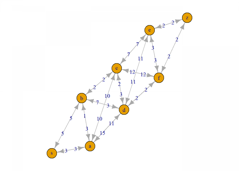
First, we are going to define the graph in which we want to navigate and we attach weights for the time it takes to cover it. We use the excellent igraph package (on CRAN) for visualizing the graph:
library(igraph)
## Attaching package: 'igraph'
## The following objects are masked from 'package:stats':
##
##     decompose, spectrum
## The following object is masked from 'package:base':
##
##     union
graph <- list(s = c("a", "b"),
              a = c("s", "b", "c", "d"),
              b = c("s", "a", "c", "d"),
              c = c("a", "b", "d", "e", "f"),
              d = c("a", "b", "c", "e", "f"),
              e = c("c", "d", "f", "z"),
              f = c("c", "d", "e", "z"),
              z = c("e", "f"))

weights <- list(s = c(3, 5),
                a = c(3, 1, 10, 11),
                b = c(5, 3, 2, 3),
                c = c(10, 2, 3, 7, 12),
                d = c(15, 7, 2, 11, 2),
                e = c(7, 11, 3, 2),
                f = c(12, 2, 3, 2),
                z = c(2, 2))

# create edgelist with weights
G <- data.frame(stack(graph), weights = stack(weights)[[1]])

set.seed(500)
el <- as.matrix(stack(graph))
g <- graph_from_edgelist(el)

oldpar <- par(mar = c(1, 1, 1, 1))
plot(g, edge.label = stack(weights)[[1]])
par(oldpar)
Next, we create a helper function to calculate the path length:
path_length <- function(path) {
  # if path is NULL return infinite length
  if (is.null(path)) return(Inf)

  # get all consecutive nodes
  pairs <- cbind(values = path[-length(path)], ind = path[-1])
  # join with G and sum over weights
  sum(merge(pairs, G)[ , "weights"])
}
And now for the core of the matter, Dijkstra’s algorithm: the general idea of the algorithm is very simple and elegant: start at the starting node and call the algorithm recursively for all nodes linked from there as new starting nodes and thereby build your path step by step. Only keep the shortest path and stop when reaching the end node (base case of the recursion). In case you reach a dead-end in between assign infinity as length (by the path_length function above).
I added a lot of documentation to the code so it is hopefully possible to understand how it works:
find_shortest_path <- function(graph, start, end, path = c()) {
  # if there are no nodes linked from current node (= dead end) return NULL
  if (is.null(graph[[start]])) return(NULL)
  # add next node to path so far
  path <- c(path, start)

  # base case of recursion: if end is reached return path
  if (start == end) return(path)

  # initialize shortest path as NULL
  shortest <- NULL
  # loop through all nodes linked from the current node (given in start)
  for (node in graph[[start]]) {
    # proceed only if linked node is not already in path
    if (!(node %in% path)) {
      # recursively call function for finding shortest path with node as start and assign it to newpath
      newpath <- find_shortest_path(graph, node, end, path)
      # if newpath is shorter than shortest so far assign newpath to shortest
      if (path_length(newpath) < path_length(shortest))
        shortest <- newpath
    }
  }
  # return shortest path
  shortest
}
Now, we can finally test the algorithm by calculating the shortest path from s to z and back:
find_shortest_path(graph, "s", "z") # via b
## [1] "s" "b" "c" "d" "f" "z"

find_shortest_path(graph, "z", "s") # back via a
## [1] "z" "f" "d" "b" "a" "s"
Note that the two routes are actually different because of the different weights in both directions (e.g. think of some construction work in one direction but not the other).
Next week we will learn how the Global Positioning System (GPS) works, so stay tuned!
UPDATE October 20, 2020
The post on GPS is now online:
“You Are Here”: Understanding How GPS Works.
Can this generalize to n nodes as asked about here: https://stackoverflow.com/questions/46001663/get-subgraph-of-shortest-path-between-n-nodes
Aren’t you satisfied with the answers given there?
hello, i have aproblem using the Algorithm, my final result when i ask for the shortest path is always NULL, don.t know why cause every step that i’ve done before seams correct. Can someone help me, please? i’d really appreciate it
thansk
I just reran the code with the latest R version 4.1.0 and everything seems fine. Without any additional info from your side, I will unfortunately not be able to help you.
Hi, there thanks for this algorithm. Would it be possible to help me out, on how to calculate the distance of the given path.
Thanks