
 One of my starting points into quantitative finance was Bernie Madoff’s fund. Back then because Bernie was in desperate need of money to keep his Ponzi scheme running there existed several so-called feeder funds.
One of them happened to approach me to offer me a once-in-a-lifetime investment opportunity. Or so it seemed. Now, there is this old saying that when something seems too good to be true it probably is. If you want to learn what Benford’s law is and how to apply it to uncover fraud, read on!
Here are Bernie’s monthly returns (you can find them here: madoff_returns.csv):
madoff_returns <- read.csv("Data/madoff_returns.csv")
equity_curve <- cumprod(c(100, (1 + madoff_returns$Return)))
plot(equity_curve, main = "Bernie's equity curve", ylab = "$", type = "l")
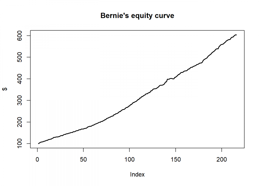
An equity curve with annual returns of over 10% as if drawn with a ruler! Wow… and Double Wow! What a hell of a fund manager!
I set off to understand how Bernie accomplished those high and especially extraordinarily stable returns. And found: Nothing! I literally rebuilt his purported split-strike strategy and backtested it (you can do the same: Backtesting Options Strategies with R), but of course, it didn’t work. And therefore, I didn’t invest with him. A wise decision as history proved. And yet, I learned so much along the way, especially on trading and options strategies.
A very good and detailed account of the Madoff fraud can be read in the excellent book “No One Would Listen: A True Financial Thriller” by whistleblower Harry Markopolos who was on Bernie’s heels for many years but as the title says, no one would listen… The reason is some variant of the above wisdom “What seems too good to be true…”: people told him that Bernie could not be a fraud because his fund was so big and other people would have realized that!
One of the red flags that those returns were made up could have been raised by applying Benford’s law. It states that the frequency of the leading digits of many real-world data sets follows a very distinct pattern:
theory <- log10(2:9) - log10(1:8)
theory <- round(c(theory, 1-sum(theory)), 3)
data.frame(theory)
##   theory
## 1  0.301
## 2  0.176
## 3  0.125
## 4  0.097
## 5  0.079
## 6  0.067
## 7  0.058
## 8  0.051
## 9  0.046
The discovery of Benford’s law goes back to 1881 when the astronomer Simon Newcomb noticed that in logarithm tables the earlier pages were much more worn than the other pages. It was re-discovered in 1938 by the physicist Frank Benford and subsequently named after him. Thereby it is just another instance of Stigler’s law which states that no scientific discovery is named after its original discoverer (Stigler’s law is by the way another instance of Stigler’s law because the idea goes back at least as far as to Mark Twain).
Thie following analysis is inspired by the great book “Analytics Stories” by my colleague Professor em. Wayne L. Winston from Kelley School of Business at Indiana University. Professor Winston gives an insightful explanation of why Benford’s law holds for many real-world data sets:
Many quantities (such as population and a company’s sales revenue) grow by a similar percentage (say, 10%) each year. If this is the case, and the first digit is a 1, it may take several years to get to a first digit of 2. If your first digit is 8 or 9, however, growing at 10% will quickly send you back to a first digit of 1. This explains why smaller first digits are more likely than larger first digits.
Let us try this idea and visualize the sequence of first digits:
start <- 100
growth <- 1.05

n <- 95
sim <- cumprod(c(start, rep(growth, (n-1)))) # vectorize recursive simulation
first_digit <- as.numeric(substr(sim, 1, 1))
sim |> round(2)
##  [1]  100.00  105.00  110.25  115.76  121.55  127.63  134.01  140.71  147.75
## [10]  155.13  162.89  171.03  179.59  188.56  197.99  207.89  218.29  229.20
## [19]  240.66  252.70  265.33  278.60  292.53  307.15  322.51  338.64  355.57
## [28]  373.35  392.01  411.61  432.19  453.80  476.49  500.32  525.33  551.60
## [37]  579.18  608.14  638.55  670.48  704.00  739.20  776.16  814.97  855.72
## [46]  898.50  943.43  990.60 1040.13 1092.13 1146.74 1204.08 1264.28 1327.49
## [55] 1393.87 1463.56 1536.74 1613.58 1694.26 1778.97 1867.92 1961.31 2059.38
## [64] 2162.35 2270.47 2383.99 2503.19 2628.35 2759.77 2897.75 3042.64 3194.77
## [73] 3354.51 3522.24 3698.35 3883.27 4077.43 4281.30 4495.37 4720.14 4956.14
## [82] 5203.95 5464.15 5737.36 6024.22 6325.44 6641.71 6973.79 7322.48 7688.61
## [91] 8073.04 8476.69 8900.52 9345.55 9812.83
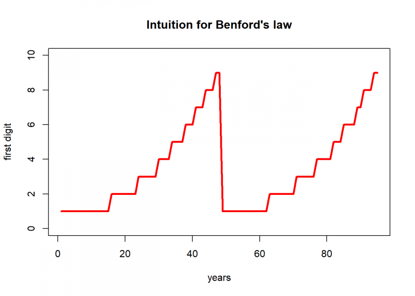
Interesting, this idea obviously has some merit to it!
Now, we are going one step further and simulate a growth process by sampling some random numbers as a starting value and a growth rate and letting it grow a few hundred times, each time extracting the first digit of the resulting number, tallying everything up, and comparing it to the above distribution at the end:
# needs dataframe with actual and theoretic distribution
plot_benford <- function(benford) {
  colours = c("red", "blue")
  bars <- t(benford)
  colnames(bars) <- 1:9
  barplot(bars, main = "Frequency analysis of first digits", xlab = "Digits", ylab = "Frequency", beside = TRUE, col = colours, ylim=c(0, max(benford) * 1.2))
  legend('topright', fill = colours, legend = c("Actual", "Theory"))
}

set.seed(123)
start <- sample(1:9000000, 1)
growth <- 1 + sample(1:50, 1) / 100

n <- 500
sim <- cumprod(c(start, rep(growth, (n-1)))) # vectorize recursive simulation
first_digit <- as.numeric(substr(sim, 1, 1))
actual <- as.vector(table(first_digit) / n)
benford_sim <- data.frame(actual, theory)
benford_sim
##   actual theory
## 1  0.300  0.301
## 2  0.174  0.176
## 3  0.126  0.125
## 4  0.098  0.097
## 5  0.078  0.079
## 6  0.068  0.067
## 7  0.058  0.058
## 8  0.050  0.051
## 9  0.048  0.046

plot_benford(benford_sim)
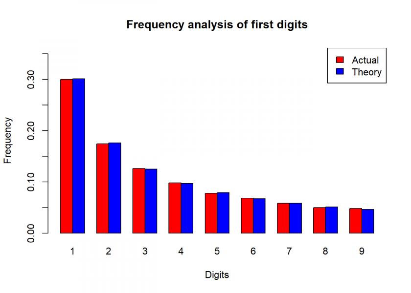
We can see a nearly perfect fit!
The resulting plot very much looks like an exponential distribution which is not that surprising given the repeated multiplicative nature of the described process. That also squares with the definition in the form of differences of logs.
We are now doing the same kind of analysis with Bernie’s made-up returns:
first_digit <- as.numeric(substr(abs(madoff_returns$Return * 10000), 1, 1))
actual <- round(as.vector(table(first_digit) / length(first_digit)), 3)
madoff <- data.frame(actual = actual[2:10], theory)
madoff
##   actual theory
## 1  0.391  0.301
## 2  0.135  0.176
## 3  0.093  0.125
## 4  0.060  0.097
## 5  0.051  0.079
## 6  0.079  0.067
## 7  0.065  0.058
## 8  0.070  0.051
## 9  0.051  0.046

plot_benford(madoff)
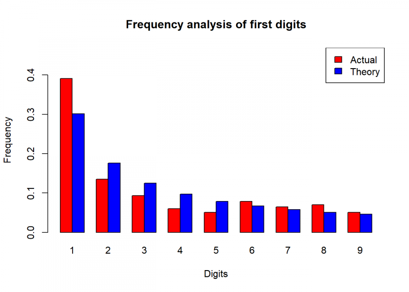
Just by inspection, we can see that something doesn’t seem to be quite right. This is of course no proof but another indication that something could be amiss.
Benford’s law has become one of the standard methods used for fraud detection, forensic analytics and forensic accounting (also called forensic accountancy or financial forensics). There are several R packages with which you can finetune the above analysis, yet the principle stays the same. Because this has become common knowledge many more sophisticated fraudsters tailor their numbers according to Benford’s law so that it may become an instance of yet another law: Goodhart’s law:
Any observed statistical regularity will tend to collapse once pressure is placed upon it for control purposes.
Let us hope that this law doesn’t lead to more lawlessness!
DISCLAIMER
This post is written on an “as is” basis for educational purposes only and comes without any warranty. The findings and interpretations are exclusively those of the author and are not endorsed by or affiliated with any third party.
In particular, this post provides no investment advice! No responsibility is taken whatsoever if you lose money.
(If you make any money though I would be happy if you would buy me a coffee… that is not too much to ask, is it? 😉 )
UPDATE January 12, 2023
I created a video for this post (in German):
You seriously can’t deny that it would have been once in a lifetime opportunity. Just not in the way that it was advertised. 🙂 Regularity related to highly successful funds, especially those employing quantitative strategies: AUM growth invariably leads to lower returns. Niches from which a small fund can extract excess returns have limited liquidity, so the fund can’t scale up its original strategy but returns get diluted. That’s why the few that outperform consistently don’t accept new capital. Bernie obviously had to fully disclose his purported trades to auditors. To my understanding, his disclosures, that were manufactured afterwards, were consistent with market quotations. But auditors didn’t check whether the actual market volume was even close to what it should have been if Bernie’s trades had actually taken place. So Bernie got away for quite some time due to the lack of basic sanity checks.
Yes, when you read the above-mentioned book you can see that there were many red flags but as the title says: no one would listen!
My backlog of books to read or listen keeps growing faster than Madoff’s equity. I’ve read “Why they do it” by Eugene Soltes. It had a chapter or two on Bernie, so it wasn’t that in-depth.
In case you want a live fund for analysis, I happen to know one with returns least as consistent as Bernie’s, but double the slope. And that’s despite they had over 30% cash (out of close to EUR 1000M AUM) last time I checked. It seems more like a quasi-Ponzi. They’ve come up with their own valuation scheme that assumes ability to hold portfolio of hard-to-sell assets to their distant maturities. Redemption ruled are quite liberal for that. They are not necessarily concealing facts or doing anything criminal. Wouldn’t want to be their auditor, though.
Seems to be an interesting title, thank you for the suggestion!
I wouldn’t want to invest in this fund…
I came across some Madoff dara a while ago, mybe the one you are discussing here. In any case, I applied Benford’s Law to the data and put my results on my blog. You can read my analysis, get the data and get my spreadsheet here: https://excelmaster.co/benford-catches-madoff/
Thank you, Duncan. Why don’t you allow comments under your posts?
Correct me if I’m wrong, but you’re comparing first digit frequency on Madoff’s returns to the frequency on the absolute values of your sample (i.e. cumprod on the second but not the first).
Benford’s law applies to growth processes across multiple orders of magnitude which Madoff’s returns are not.
Thank you for your comment, Stefan.
Actually, I don’t quite understand what you mean. I compare the first digit frequency of Madoff’s returns to the theoretical first digit frequency given by Benford’s law. This is standard practice in financial forensics because more than 90% of all fund returns conform to this law.
The only criticism that has, in my opinion, some merit to it is that this alone is of course not sufficient evidence to “prove” fraud, but it is certainly a red flag that calls for further investigations. Especially when returns are abnormally high over a substantial period of time as in this case.
Very neat application of Benford’s law. The problem I see with much of these types of case studies is that it only confirms what we already know – i.e. Madoff was a fraud. It’s a bit more difficult to have done this study beforehand, and then look at the Frequency Analysis of First Digits chart you have above, and then decide that the chart indicates fraud. How much of a mismatch is ok? Some people are talking about applying this law to voting returns in the recent US election, and the comparison to Benford’s law does seem to show some mismatch to theory in some limited cases, but then others state that such a result is not unexpected, and does not indicate fraud at all. What might be interesting would be some A/B test method for calculating the probability that the results are unexpected, given X disparity from Benford’s law…
Thank you for your feedback, I appreciate it.
Well, I think there are all kinds of statistical tests out there but the main problem remains that this is of course not sufficient evidence. There will be both kinds of errors (false positive and false negative). On top of that people can manipulate returns so that they look like real returns, including conforming to Benford’s law.
I think Stefan refers to Winston’s explanation on origin of the “law”. Equity is a growth process. The theory implies that sampling equity values from long enough time series should reproduce Benford’s distribution. But there’s no apparent explanation why short-term (monthly) returns should behave similarly, even though it can be an empirical fact. But I’m not sure how do you arrive at 90%. What’s the sample, and how do you classify the individual instances in it to conforming and non-conforming (the remaining 10%)?
Ah, ok, I understand. For the 90+% see e.g. here: https://michaelsinkey.files.wordpress.com/2016/12/bmss_09_20161.pdf.
Thanks, will need some time to digest that. Going slightly off-topic, now would be great occasion to write about quantitative measures of vaccine efficacy. Headlines are telling us that some vaccine is 90% or 95% percent effective. But what does such number actually tell you? Does it indicate that 9x% of recipients become immune to the disease? (answer: no) Or does it state that a vaccinated person has risk of developing the disease reduced by 9x% after single exposure? (answer: no, but getting closer) Does it indicate how a vaccination program will change the basic reproductive number? (answer: in essence, yes!)
Wow, Lauri, now you got me!
I know that you sent me a draft of your article on stable distributions already (thank you for that!) but this topic would really be a scoop!
As you will know, I have a COVID-19 section here: https://blog.ephorie.de/category/covid-19. If you could write a guest post on some vaccine stats I would immediately publish it!