Learning Data Science: Understanding and Using k-means Clustering

A few months ago I published a quite popular post on Clustering the Bible… one well known clustering algorithm is k-means. If you want to learn how k-means works and how to apply it in a real-world example, read on…

k-means (not to be confused with k-nearest neighbours or KNN: Teach R to read handwritten Digits with just 4 Lines of Code) is a simple, yet often very effective unsupervised learning algorithm to find similarities in large amounts of data and cluster them accordingly. The hyperparameter k stands for the number of clusters which has to be set beforehand.

The guiding principles are:

• The distance between data points within clusters should be as small as possible.
• The distance of the centroids (= centres of the clusters) should be as big as possible.

Because there are too many possible combinations of all possible clusters comprising all possible data points k-means follows an iterative approach:

1. Initialization: assign all data points randomly to k clusters
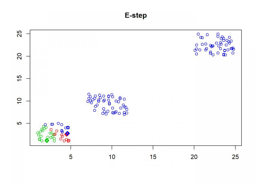
2. E-step (for expectation): assign each point to the nearest (based on Euclidean distance) centroid
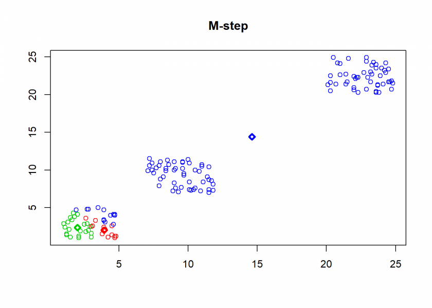
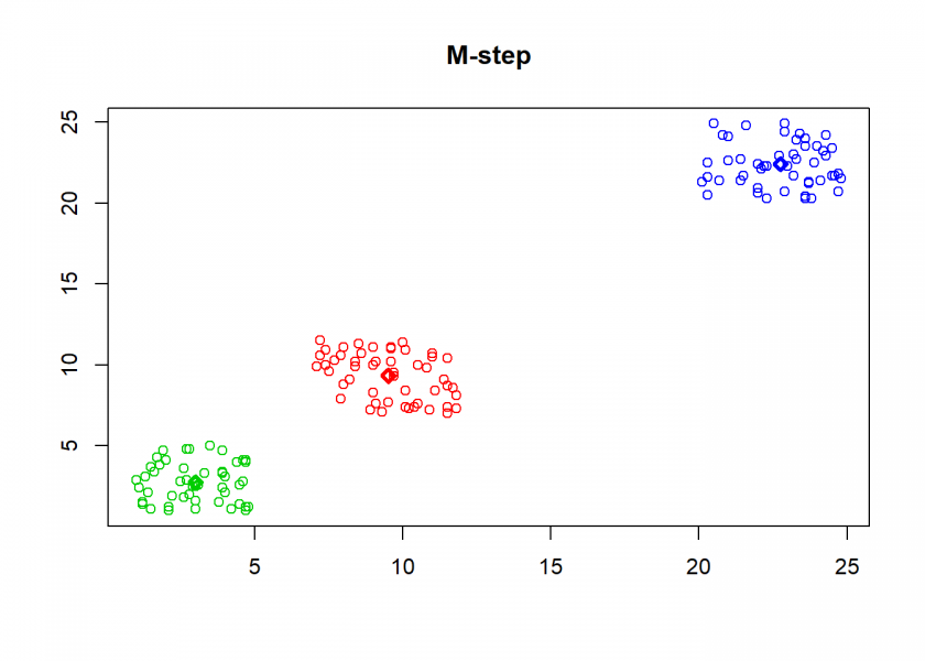
3. M-step (for maximization): determine new centroids based on the mean of all assigned points
4. Repeat steps 2 and 3 until no further changes occur

As can be seen above k-means is an example of a so-called expectation-maximization algorithm.

To implement k-means in R we first assign some variables and define a helper function for plotting the steps:

n <- 3 # no. of centroids
set.seed(1415) # set seed for reproducibility

M1 <- matrix(round(runif(100, 1, 5), 1), ncol = 2)
M2 <- matrix(round(runif(100, 7, 12), 1), ncol = 2)
M3 <- matrix(round(runif(100, 20, 25), 1), ncol = 2)
M <- rbind(M1, M2, M3)

C <- M[1:n, ] # define centroids as first n objects
obs <- length(M) / 2
A <- sample(1:n, obs, replace = TRUE) # assign objects to centroids at random
colors <- seq(10, 200, 25) 

clusterplot <- function(M, C, txt) {
  plot(M, main = txt, xlab = "", ylab = "")
  for(i in 1:n) {
    points(C[i, , drop = FALSE], pch = 23, lwd = 3, col = colors[i])
    points(M[A == i, , drop = FALSE], col = colors[i])    
  }
}
clusterplot(M, C, "Initialization")

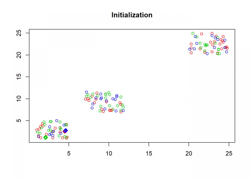
Here comes the k-means algorithm as described above (the circles are the data points, diamonds are the centroids and the three colours symbolize cluster assignments):

repeat {
  # calculate Euclidean distance between objects and centroids
  D <- matrix(data = NA, nrow = n, ncol = obs)
  for(i in 1:n) {
    for(j in 1:obs) {
      D[i, j] <- sqrt((M[j, 1] - C[i, 1])^2 + (M[j, 2] - C[i, 2])^2)
    }
  }
  O <- A
  
  ## E-step: parameters are fixed, distributions are optimized
  A <- max.col(t(-D)) # assign objects to centroids
  if(all(O == A)) break # if no change stop
  clusterplot(M, C, "E-step")
  
  ## M-step: distributions are fixed, parameters are optimized
  # determine new centroids based on mean of assigned objects
  for(i in 1:n) {
    C[i, ] <- apply(M[A == i, , drop = FALSE], 2, mean)
  }
  clusterplot(M, C, "M-step")
}

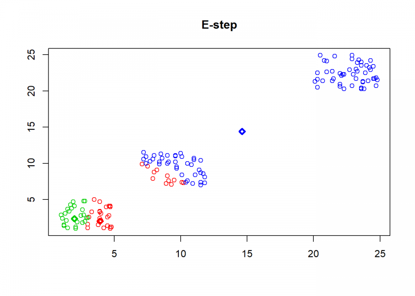
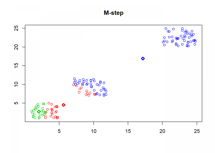
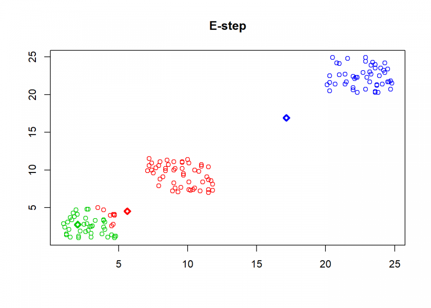
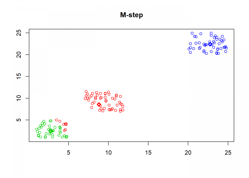
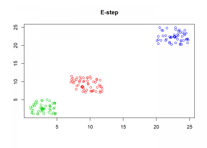
As can seen the clusters wander slowly but surely until all three are stable. We now compare the result with the k-means function in Base R:

cl <- kmeans(M, n)
clusterplot(M, cl$centers, "Base R")

(custom <- C[order(C[ , 1]), ])
##        [,1]   [,2]
## [1,]  3.008  2.740
## [2,]  9.518  9.326
## [3,] 22.754 22.396

(base <- cl$centers[order(cl$centers[ , 1]), ])
##     [,1]   [,2]
## 2  3.008  2.740
## 1  9.518  9.326
## 3 22.754 22.396

round(base - custom, 13)
##   [,1] [,2]
## 2    0    0
## 1    0    0
## 3    0    0

As you can see, the result is the same!

Now, for some real-world application: clustering wholesale customer data. The data set refers to clients of a wholesale distributor. It includes the annual spending on diverse product categories and is from the renowned UCI Machine Learning Repository (I guess the category “Delicassen” should rather be “Delicatessen”).

Have a look at the following code:

data <- read.csv("https://archive.ics.uci.edu/ml/machine-learning-databases/00292/Wholesale customers data.csv", header = TRUE)
head(data)
##   Channel Region Fresh Milk Grocery Frozen Detergents_Paper Delicassen
## 1       2      3 12669 9656    7561    214             2674       1338
## 2       2      3  7057 9810    9568   1762             3293       1776
## 3       2      3  6353 8808    7684   2405             3516       7844
## 4       1      3 13265 1196    4221   6404              507       1788
## 5       2      3 22615 5410    7198   3915             1777       5185
## 6       2      3  9413 8259    5126    666             1795       1451

set.seed(123)
k <- kmeans(data[ , -c(1, 2)], centers = 4) # remove columns 1 and 2, create 4 clusters
(centers <- k$centers) # display cluster centers
##       Fresh      Milk   Grocery   Frozen Detergents_Paper Delicassen
## 1  8149.837 18715.857 27756.592 2034.714        12523.020   2282.143
## 2 20598.389  3789.425  5027.274 3993.540         1120.142   1638.398
## 3 48777.375  6607.375  6197.792 9462.792          932.125   4435.333
## 4  5442.969  4120.071  5597.087 2258.157         1989.299   1053.272

round(prop.table(centers, 2) * 100) # percentage of sales per category
##   Fresh Milk Grocery Frozen Detergents_Paper Delicassen
## 1    10   56      62     11               76         24
## 2    25   11      11     22                7         17
## 3    59   20      14     53                6         47
## 4     7   12      13     13               12         11

table(k$cluster) # number of customers per cluster
## 
##   1   2   3   4 
##  49 113  24 254

One interpretation could be the following for the four clusters:

1. Big general shops
2. Small food shops
3. Big food shops
4. Small general shops

As you can see, the interpretation of some clusters found by the algorithm can be quite a challenge. If you have a better idea of how to interpret the result please tell me in the comments below!