

What is the best way for me to find out whether you are rich or poor, when the only thing I know is your address? Looking at your neighbourhood! That is the big idea behind the k-nearest neighbours (or KNN) algorithm, where k stands for the number of neighbours to look at. The idea couldn’t be any simpler yet the results are often very impressive indeed – so read on…
Let us take a task that is very hard to code, like identifying handwritten numbers. We will be using the Semeion Handwritten Digit Data Set from the UCI Machine Learning Repository and are separating training and test set for the upcoming task in the first step:
# helper function for plotting images of digits in a nice way + returning the respective number
plot_digit <- function(digit) {
  M <- matrix(as.numeric(digit[1:256]), nrow = 16, ncol = 16, byrow = TRUE)
  image(t(M[nrow(M):1, ]), col = c(0,1), xaxt = "n", yaxt = "n", useRaster = TRUE)
  digit[257]
}

# load data and chose some digits as examples
semeion <- read.table("data/semeion.data", quote = "\"", comment.char = "") # put in right path here!
digit_data <- semeion[ , 1:256]
which_digit <- apply(semeion[ , 257:266], 1, function(x) which.max(x) - 1)
semeion_new <- cbind(digit_data, which_digit)

# chose training and test set by chance
set.seed(123) # for reproducibility
data <- semeion_new
random <- sample(1:nrow(data), 0.8 * nrow(data)) # 80%: training data, 20%: test data
train <- data[random, ]
test <- data[-random, ]

# plot example digits
old_par <- par(mfrow = c(4, 6), oma = c(5, 4, 0, 0) + 0.1, mar = c(0, 0, 1, 1) + 0.1)
matrix(apply(train[1:24, ], 1, plot_digit), 4, 6, byrow = TRUE)
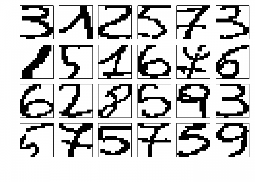
##      [,1] [,2] [,3] [,4] [,5] [,6]
## [1,]    3    1    2    5    7    3
## [2,]    1    5    1    6    7    6
## [3,]    6    2    8    5    9    3
## [4,]    5    7    5    7    5    9

par(old_par)
As you can see teaching a computer to read those digits is a task that would take considerable effort and easily hundreds of lines of code. You would have to intelligently identify different regions in the images and find some boundaries to try to identify which number is being shown. You could expect to do a lot of tweaking before you would get acceptable results.
The real magic behind machine learning and artificial intelligence is that when something is too complicated to code let the machine program itself by just showing it lots of examples (see also my post So, what is AI really?). We will do just that with the nearest neighbour algorithm.
When talking about neighbours it is implied already that we need some kind of distance metric to define what constitutes a neighbour. As in real life, the simplest one is the so-called Euclidean distance which is just how far different points are apart from each other as the crow flies. The simple formula that is used for this is just the good old Pythagorean theorem (in this case in a vectorized way) – you can see what maths at school was good for after all:
dist_eucl <- function(x1, x2) {
  sqrt(sum((x1 - x2) ^ 2)) # Pythagorean theorem!
}
The k-nearest neighbours algorithm is pretty straight forward: it just compares the digit which is to be identified with all other digits and choses the k nearest ones. In case that the k nearest ones don’t come up with the same answer the majority vote (or mathematically the mode) is taken:
mode <- function(NNs) {
  names(sort(-table(NNs[ncol(NNs)])))[1] # mode = majority vote
}
knn <- function(train, test, k = 5) {
  dist_sort <- order(apply(train[-ncol(train)], 1, function(x) dist_eucl(as.numeric(x), x2 = as.numeric(test[-ncol(test)]))))
  mode(train[dist_sort[1:k], ])
}
So, the algorithm itself comprises barely 4 lines of code! Now, let us see how it performs on this complicated task with k = 9 out of sample (first a few examples are shown and after that we have a look at the overall performance):
# show a few examples
set.seed(123) # for reproducibility
no_examples <- 24
examples <- sample(dim(test)[1], no_examples)
old_par <- par(mfrow = c(4, 6), oma = c(5, 4, 0, 0) + 0.1, mar = c(0, 0, 1, 1) + 0.1)
matrix(apply(test[examples, ], 1, plot_digit), 4, 6, byrow = TRUE)
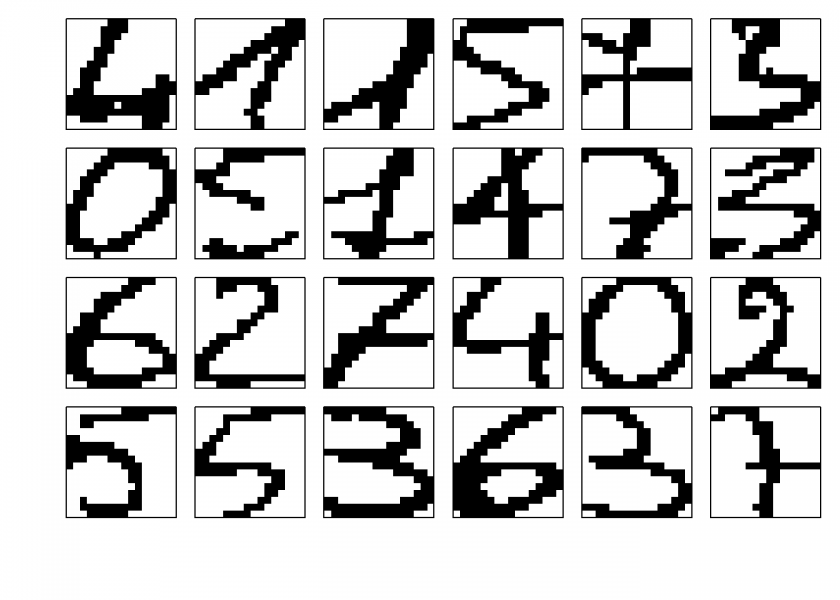
##      [,1] [,2] [,3] [,4] [,5] [,6]
## [1,]    4    1    1    5    7    3
## [2,]    0    5    1    4    7    3
## [3,]    6    2    7    4    0    2
## [4,]    5    5    3    6    3    7

par(old_par)
prediction <- integer(no_examples)
for (i in 1:no_examples) {
  prediction[i] <- knn(train, test[examples[i], ], k = 9)
}
print(matrix(prediction, 4, 6, byrow = TRUE), quote = FALSE, right = TRUE)
##      [,1] [,2] [,3] [,4] [,5] [,6]
## [1,]    4    1    1    5    7    3
## [2,]    0    5    1    4    7    3
## [3,]    6    2    7    4    0    2
## [4,]    5    5    3    6    3    7

# now for the overall accuracy
library(OneR) # just for eval_model function to evaluate the model's accuracy

prediction <- integer(nrow(test))

ptm <- proc.time()
for (i in 1:nrow(test)) {
  prediction[i] <- knn(train, test[i, ], k = 9)
}
proc.time() - ptm
##    user  system elapsed
##   26.74    0.82   27.59

eval_model(prediction, test[ncol(test)], zero.print = ".")
##
## Confusion matrix (absolute):
##           Actual
## Prediction   0   1   2   3   4   5   6   7   8   9 Sum
##        0    34   .   .   .   .   .   1   .   .   .  35
##        1     .  36   1   .   2   .   .   1   .   1  41
##        2     .   .  36   .   .   .   .   .   1   1  38
##        3     .   1   .  32   .   .   .   .   .   2  35
##        4     .   .   .   .  29   .   .   .   .   .  29
##        5     .   .   .   .   .  35   2   .   1   .  38
##        6     .   .   .   .   .   1  23   .   .   .  24
##        7     .   .   .   .   .   .   .  22   .   1  23
##        8     .   .   .   .   .   .   .   .  31   .  31
##        9     .   .   .   .   .   .   .   .   2  23  25
##        Sum  34  37  37  32  31  36  26  23  35  28 319
##
## Confusion matrix (relative):
##           Actual
## Prediction    0    1    2    3    4    5    6    7    8    9  Sum
##        0   0.11    .    .    .    .    .    .    .    .    . 0.11
##        1      . 0.11    .    . 0.01    .    .    .    .    . 0.13
##        2      .    . 0.11    .    .    .    .    .    .    . 0.12
##        3      .    .    . 0.10    .    .    .    .    . 0.01 0.11
##        4      .    .    .    . 0.09    .    .    .    .    . 0.09
##        5      .    .    .    .    . 0.11 0.01    .    .    . 0.12
##        6      .    .    .    .    .    . 0.07    .    .    . 0.08
##        7      .    .    .    .    .    .    . 0.07    .    . 0.07
##        8      .    .    .    .    .    .    .    . 0.10    . 0.10
##        9      .    .    .    .    .    .    .    . 0.01 0.07 0.08
##        Sum 0.11 0.12 0.12 0.10 0.10 0.11 0.08 0.07 0.11 0.09 1.00
##
## Accuracy:
## 0.9436 (301/319)
##
## Error rate:
## 0.0564 (18/319)
##
## Error rate reduction (vs. base rate):
## 0.9362 (p-value < 2.2e-16)
Wow, it achieves an accuracy of nearly 95% out of the box while some of the digits are really hard to read even for humans! And we haven’t even given it the information that those images are two-dimensional because we coded all the images simply as (one-dimensional) binary numbers.
To get the idea where it failed have a look at the digits that were misclassified:
# show misclassified digits
err <- which(as.integer(prediction) != unlist(test[ncol(test)]))
old_par <- par(mfrow = c(3, 6), oma = c(5, 4, 0, 0) + 0.1, mar = c(0, 0, 1, 1) + 0.1)
matrix(apply(test[err, ], 1, plot_digit), 3, 6, byrow = TRUE)
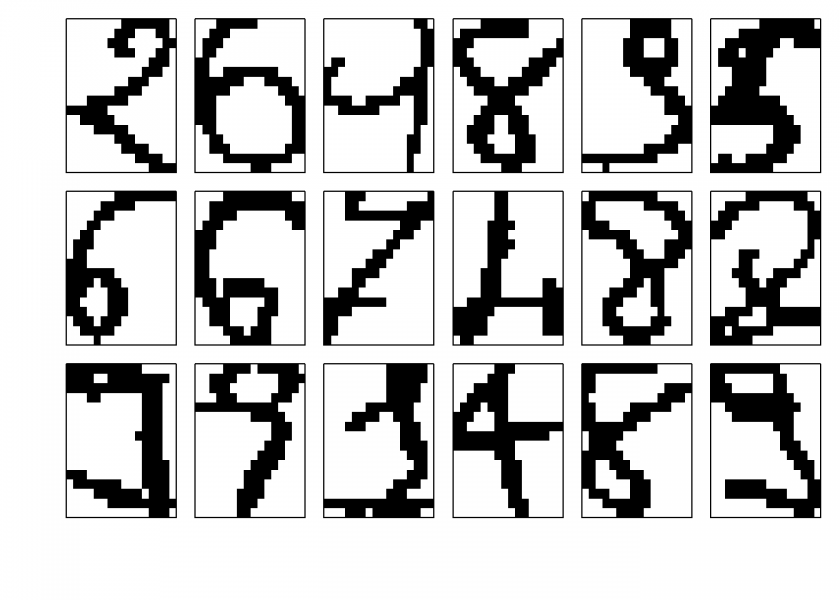
##      [,1] [,2] [,3] [,4] [,5] [,6]
## [1,]    2    6    9    8    9    5
## [2,]    6    6    7    4    8    8
## [3,]    9    9    1    4    8    9

par(old_par)

# show what was predicted
print(matrix(prediction[err], 3, 6, byrow = TRUE), quote = FALSE, right = TRUE)
##      [,1] [,2] [,3] [,4] [,5] [,6]
## [1,]    1    5    1    9    3    6
## [2,]    5    0    1    1    9    5
## [3,]    3    7    3    1    2    2
Most of us would have difficulties reading at least some of those digits too, e.g. the third digit in the first row is supposed to be a 9, yet it could also be a distorted 1 – same with the first digit in the last row: some people would read a 3 (like our little program) or nothing at all really, but it is supposed to be a 9. So even the mistakes the system makes are understandable.
Sometimes the simplest methods are – perhaps not the best but – very effective indeed, you should keep that in mind!
Wonderful article. Thanks.
Looks like the KNN function is missing a closing “}” Other than that, it works wonderfully.
Thank you, Tim! I fixed it.
Something I’ve always wondered about number recognition but never got around to exploring, how does R handle multiple numbers? Can it recognize “9” vs “91” vs “8000”? I imagine not with this code here, but in some fashion?
Well, R per se doesn’t do anything, you have to program something into it or use a package which does it for you. One possibility is that you preprocess the numbers to separate the digits and after that identify them one by one, e.g. as seen above or with a neural network (see Understanding the Magic of Neural Networks).
Or did I misunderstand your question?