

Everything “neural” is (again) the latest craze in machine learning and artificial intelligence. Now what is the magic of artificial neural networks (ANNs)?
Let us dive directly into a (supposedly little silly) example: we have three protagonists in the fairy tale little red riding hood, the wolf, the grandmother, and the woodcutter. They all have certain qualities and little red riding hood reacts in certain ways towards them. For example the grandmother has big eyes, is kindly and wrinkled – little red riding hood will approach her, talk to her and offer her food (the example is based on Jones, W. & Hoskins, J.: Back-Propagation, Byte, 1987). We will build and train an artificial neural network that gets the qualities as inputs and little red riding hood’s behaviour as output, i.e. we train it to learn the adequate behaviour for each quality.
Have a look at the following code and its output including the resulting plot:
library(neuralnet)
library(NeuralNetTools)

# code qualities and actions
qualities <- matrix (c(1, 1, 1, 0, 0, 0,
                       0, 1, 0, 1, 1, 0,
                       1, 0, 0, 1, 0, 1), byrow = TRUE, nrow = 3)
colnames(qualities) <- c("big_ears", "big_eyes", "big_teeth", "kindly", "wrinkled", "handsome")
rownames(qualities) <- c("wolf", "grannie", "woodcutter")
qualities
##            big_ears big_eyes big_teeth kindly wrinkled handsome
## wolf              1        1         1      0        0        0
## grannie           0        1         0      1        1        0
## woodcutter        1        0         0      1        0        1

actions <- matrix (c(1, 1, 1, 0, 0, 0, 0,
                     0, 0, 0, 1, 1, 1, 0,
                     0, 0, 0, 1, 0, 1, 1), byrow = TRUE, nrow = 3)
colnames(actions) <- c("run_away", "scream", "look_for_woodcutter", "talk_to", "approach", "offer_food", "is_rescued_by")
rownames(actions) <- rownames(qualities)
actions
##            run_away scream look_for_woodcutter talk_to approach offer_food
## wolf              1      1                   1       0        0          0
## grannie           0      0                   0       1        1          1
## woodcutter        0      0                   0       1        0          1
##            is_rescued_by
## wolf                   0
## grannie                0
## woodcutter             1
data <- cbind(qualities, actions)

# train the neural network (NN)
set.seed(123) # for reproducibility
neuralnetwork <- neuralnet(run_away + scream + look_for_woodcutter + talk_to + approach +
                             offer_food + is_rescued_by ~
                             big_ears + big_eyes + big_teeth + kindly + wrinkled + handsome,
                           data = data, hidden = 3, exclude = c(1, 8, 15, 22, 26, 30, 34, 38, 42, 46),
                           lifesign = "minimal", linear.output = FALSE)
## hidden: 3    thresh: 0.01    rep: 1/1    steps:      48  error: 0.01319  time: 0.01 secs

# plot the NN
par_bkp <- par(mar = c(0, 0, 0, 0)) # set different margin to minimize cutoff text
plotnet(neuralnetwork, bias = FALSE)
par(par_bkp)

# which actions were learned by the net?
round(neuralnetwork$net.result[[1]])
##            [,1] [,2] [,3] [,4] [,5] [,6] [,7]
## wolf          1    1    1    0    0    0    0
## grannie       0    0    0    1    1    1    0
## woodcutter    0    0    0    1    0    1    1
First, the qualities and actions are coded as binary variables in a data frame. After that, the neural network is being trained with the qualities as input and the resulting behaviour as output (using the standard formula syntax). In the neuralnet function, a few additional technical arguments are set which details won’t concern us here, they just simplify the process in this context). Then we plot the learned net and test it by providing it with the respective qualities: in all three cases it learned the right actions. How did it achieve that?
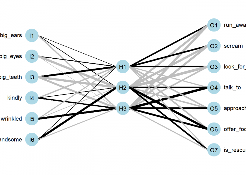
Let us look at the plot of the net. We see that there are two basic building blocks: neurons and weighted connections between them. We have one neuron for each quality and one neuron for each action. Between both layers we have a so-called hidden layer with three neurons in this case. The learned strength between the neurons is shown by the thickness of the lines (whereby ‘black’ means positive and ‘grey’ negative weights). Please have a thorough look at those weights.
You might have noticed that although the net didn’t know anything about the three protagonists in our little story it nevertheless correctly built a representation of them: ‘H1’ (for Hidden 1) represents the wolf because its differentiating quality is ‘big teeth’ which leads to ‘run away’, ‘scream’ and ‘look for woodcutter’, by the same logic ‘H2’ is the woodcutter and ‘H3’ is the grandmother (quite literally the infamous ‘grandmother neuron’!). So, the net learned to connect the qualities with the respective actions of little red riding hood by creating a representation of the three protagonists! It learned a representation of its little world; it built a world model!
So, an artificial neural network is obviously a network of neurons… so let us have a look at those neurons! Basically, they are mathematical abstractions of real neurons in your brain. They consist of inputs and an output. The biologically inspired idea is that when the activation of the inputs surpasses a certain threshold the neuron fires. To be able to learn the neuron must, before summing up the inputs, adjust the inputs so that the output is not just arbitrary but matches some sensible result. What is ‘sensible’, you might ask? In a biological environment, the answer is not always so clear cut but in our simple example here the neuron has just to match the output we provide it with (= supervised learning).
The following abstraction has all we need, inputs, weights, the sum function, a threshold after that and finally the output of the neuron:

Let us talk a little bit about what is going on here intuitively. First, every input is taken, multiplied by its weight and all of this is summed up. Some of you might recognize this mathematical operation as a scalar product (also called dot product). Another mathematical definition of a scalar product is the following:
![\[\mathbf{a}\cdot\mathbf{b}=\|\mathbf{a}\|\ \|\mathbf{b}\|\cos(\theta)\]](https://blog.ephorie.de/wp-content/ql-cache/quicklatex.com-812a5d4a84f437f7861280fe8cdac010_l3.png "Rendered by QuickLaTeX.com")
That is we multiply the length of two vectors by the cosine of the angle of those two vectors. What has cosine to do with it? The cosine of an angle becomes one when both vectors point in the same direction, it becomes zero when they are orthogonal and minus one when both point into opposite directions. Does this make sense? Well, I give you a little (albeit crude) parable. When growing up there are basically three stages: first you are totally dependent on your parents, then comes puberty and you are against whatever they say or think and after some years you are truly independent (some never reach that stage…). What does “independent” mean here? It means that you agree with some of the things your parents say and think and you disagree with some other things. During puberty you are as dependent on your parents as during being a toddler – you just don’t realize that but in reality you, so to speak, only multiply everything your parents say or think times minus one!
What is the connection with cosine? Well, as a toddler both you and your parents tend to be aligned which gives one, during puberty both of you are aligned but in opposing directions which gives minus one and only as a grown-up you are both independent which mathematically means that your vector in a way points in both directions at the same time which is only possible when it is orthogonal on the vector of your parents (you entered a new dimension, literally) – and that gives zero for the cosine.
So cosine is nothing but a measure of dependence – as is correlation by the way. So this setup ensures that the neuron learns the dependence (or correlation) structure between the inputs and the output! The step function is just a way to help it to decide on which side of the fence it wants to sit, to make the decision clearer whether to fire or not. To sum it up, an artificial neuron is a non-linear function (in this case a step function) on a scalar product of the inputs (fixed) and the weights (adaptable to be able to learn). By adapting the weights the neuron learns the dependence structure between inputs and output.
In R you code this idea of an artificial neuron as follows:
neuron <- function(input) ifelse(weights %*% input > 0, 1, 0)
Now let us use this idea in R by training an artificial neuron to classify points in a plane. Have a look at the following table:
| Input 1 | Input 2 | Output |
|---|---|---|
| 1 | 0 | 0 |
| 0 | 0 | 1 |
| 1 | 1 | 0 |
| 0 | 1 | 1 |
If you plot those points with the colour coded pattern you get the following picture:
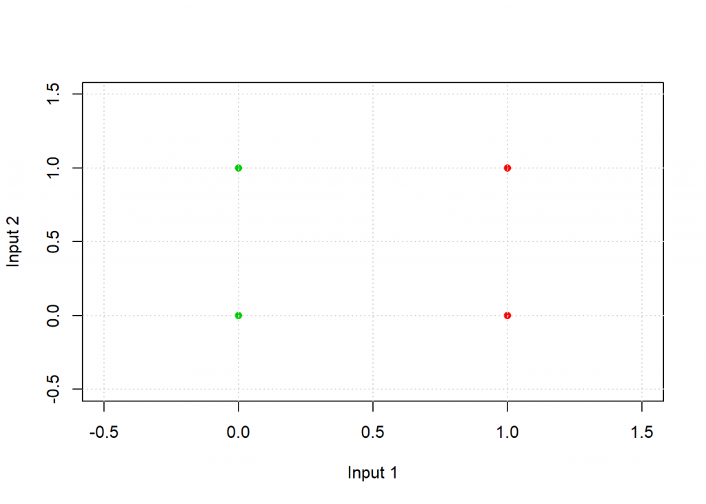
The task for the neuron is to find a separating line and thereby classify the two groups. Have a look at the following code:
# inspired by Kubat: An Introduction to Machine Learning, p. 72
plot_line <- function(w, col = "blue", add = TRUE)
  curve(-w[1] / w[2] * x - w[3] / w[2], xlim = c(-0.5, 1.5), ylim = c(-0.5, 1.5), col = col, lwd = 3, xlab = "Input 1", ylab = "Input 2", add = add)
neuron <- function(input) as.vector(ifelse(input %*% weights > 0, 1, 0)) # step function on scalar product of weights and input
eta <- 0.5 # learning rate

# examples
input <- matrix(c(1, 0,
                  0, 0,
                  1, 1,
                  0, 1), ncol = 2, byrow = TRUE)
input <- cbind(input, 1) # bias for intercept of line
output <- c(0, 1, 0, 1)
weights <- c(0.25, 0.2, 0.35) # random initial weights

plot_line(weights, add = FALSE); grid()
points(input[ , 1:2], pch = 16, col = (output + 2))

# training of weights of neuron
for (example in 1:length(output)) {
  weights <- weights + eta * (output[example] - neuron(input[example, ])) * input[example, ]
  plot_line(weights)
}
plot_line(weights, col = "black")
# test: applying neuron on input
apply(input, 1, neuron)
## [1] 0 1 0 1
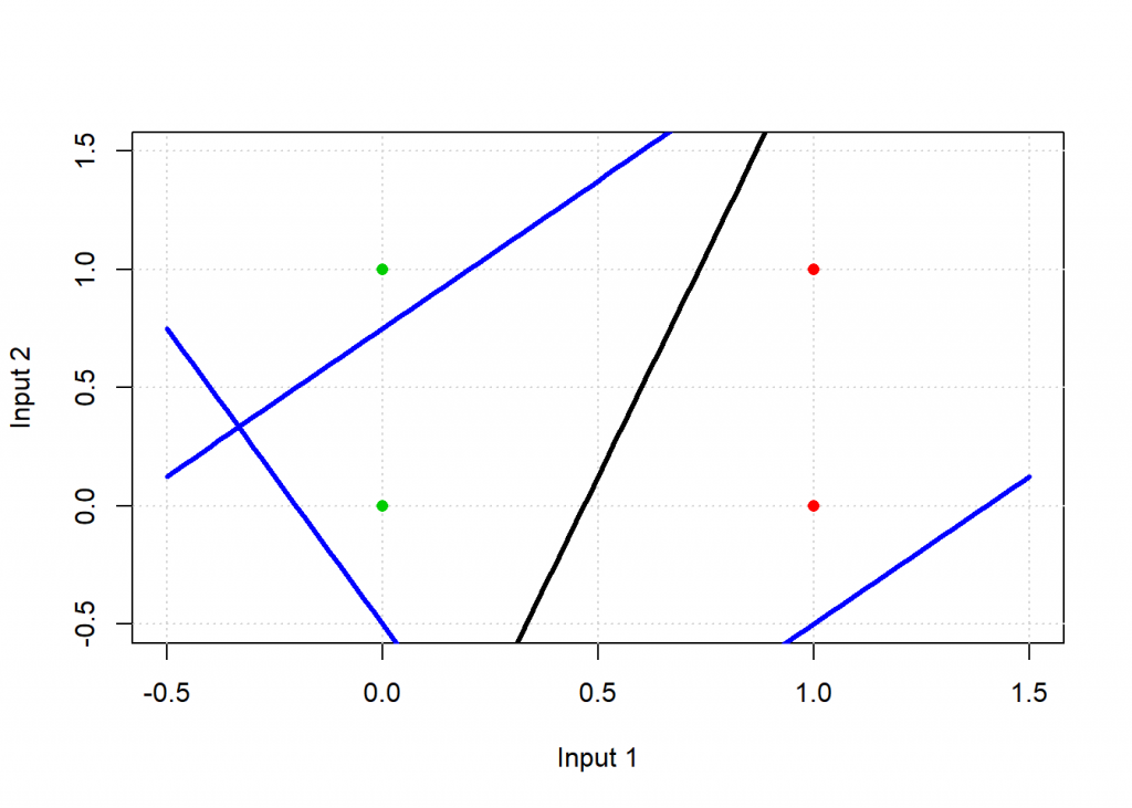
As you can see the result matches the desired output, graphically the black line is the end result and as you can see it separates the green from the red points: the neuron has learned this simple classification task. The blue lines are where the neuron starts from and where it is during training – they are not able to classify the points correctly.
The training, i.e. adapting the weights, takes places in this line:
weights <- weights + eta * (output[example] - neuron(input[example, ])) * input[example, ]
The idea is to compare the current output of the neuron with the wanted output, scale that by some learning factor  (eta) and modify the weights accordingly. So if the output is too big make the weights smaller and vice versa. Do this for all examples (sometimes you need another loop to train the neuron with the examples several times) and that’s it. That is the core idea behind the ongoing revolution of neural networks!
(To understand just another fascinating interpretation of the core of neural networks see also this post: Logistic Regression as the Smallest Possible Neural Network.)
Ok, so far we had a closer look at the core part of neural networks, namely the neurons, let us now turn to the network structure (also called network topology). First, why do we need a whole network anyway when the neurons are already able to solve classification tasks? The answer is that they can do that only for very simple problems. For example, the neuron above can only distinguish between linearly separable points, i.e. it can only draw lines. It fails in case of the simple problem of four points that are coloured green, red, red, green from top left to bottom right (try it yourself). We would need a non-linear function to separate the points. We have to combine several neurons to solve more complicated problems.
The biggest problem you have to overcome when you combine several neurons is how to adapt all the weights. You need a system of how to attribute the error at the output layer to all the weights in the net. This had been a profound obstacle until an algorithm called backpropagation (also abbreviated backprop) was invented (or found). We won’t get into the details here but the general idea is to work backwards from the output layers through all of the hidden layers till one reaches the input layer and modify the weights according to their respective contribution to the resulting error. This is done several (sometimes millions of times) for all training examples until one achieves an acceptable error rate for the training data.
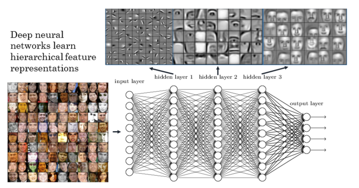
The result is that you get several layers of abstraction, so when you e.g. want to train a neural network to recognize certain faces you start with the raw input data in the form of pixels, these are automatically combined into abstract geometrical structures, after that the net detects certain elements of faces, like eyes and noses, and finally abstractions of certain faces are being rebuilt by the net. See the following picture for an illustration:
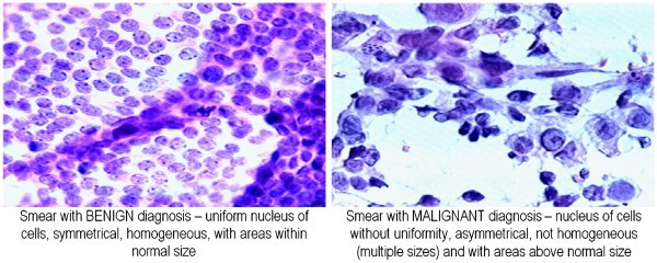
So far we have only coded very small examples of neural networks. Real-world examples often have dozens of layers with thousands of neurons so that much more complicated patterns can be learned. The more layers there are the ‘deeper’ a net becomes… which is the reason why the current revolution in this field is called “deep learning” because there are so many hidden layers involved. Let us now look at a more realistic example: predicting whether a breast cell is malignant or benign.
Have a look at the following code:
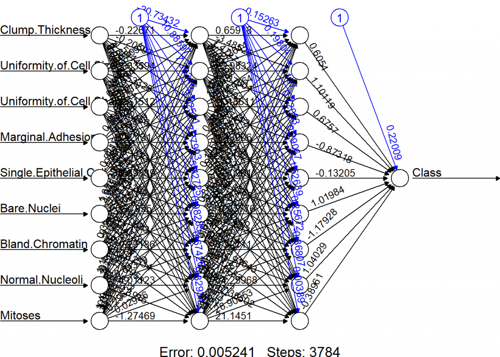
library(OneR)
data(breastcancer)
data <- breastcancer
colnames(data) <- make.names(colnames(data))
data$Class <- as.integer(as.numeric(data$Class) - 1) # for compatibility with neuralnet
data <- na.omit(data)

# Divide training (80%) and test set (20%)
set.seed(12) # for reproducibility
random <- sample(1:nrow(data), 0.8 * nrow(data))
data_train <- data[random, ]
data_test <- data[-random, ]

# Train NN on training set
model_train <- neuralnet(Class ~., data = data_train, hidden = c(9, 9), lifesign = "minimal")
## hidden: 9, 9    thresh: 0.01    rep: 1/1    steps:    3784   error: 0.00524  time: 3.13 secs

# Plot net
plot(model_train, rep = "best")
# Use trained model to predict test set
prediction <- round(predict(model_train, data_test))
eval_model(prediction, data_test)
##
## Confusion matrix (absolute):
##           Actual
## Prediction   0   1 Sum
##        0    93   2  95
##        1     4  38  42
##        Sum  97  40 137
##
## Confusion matrix (relative):
##           Actual
## Prediction    0    1  Sum
##        0   0.68 0.01 0.69
##        1   0.03 0.28 0.31
##        Sum 0.71 0.29 1.00
##
## Accuracy:
## 0.9562 (131/137)
##
## Error rate:
## 0.0438 (6/137)
##
## Error rate reduction (vs. base rate):
## 0.85 (p-value = 1.298e-13)
So you see that a relatively simple net achieves an accuracy of about 95% out of sample. The code itself should be mostly self-explanatory. For the actual training the neuralnet function from the package with the same name is being used, the input method is the standard R formula interface, where you define Class as the variable to be predicted by using all the other variables (coded as .~).
When you look at the net one thing might strike you as odd: there are three neurons at the top with a fixed value of 1. These are so-called bias neurons and they serve a similar purpose as the intercept in a linear regression: they kind of shift the model as a whole in n-dimensional feature space just as a regression line is being shifted by the intercept. In case you were attentive we also smuggled in a bias neuron in the above example of a single neuron: it is the last column of the input matrix which contains only ones.
Another thing: as can even be seen in this simple example it is very hard to find out what a neural network has actually learned – the following well-known anecdote (urban legend?) shall serve as a warning: some time ago the military built a system which had the aim to distinguish military vehicles from civilian ones. They chose a neural network approach and trained the system with pictures of tanks, humvees and missile launchers on the one hand and normal cars, pickups and lorries on the other. After having reached a satisfactory accuracy they brought the system into the field (quite literally). It failed completely, performing no better than a coin toss. What had happened? No one knew, so they re-engineered the black box (no small feat in itself) and found that most of the military pics were taken at dusk or dawn and most civilian pics under brighter weather conditions. The neural net had learned the difference between light and dark!
Just for comparison the same example with the OneR package:
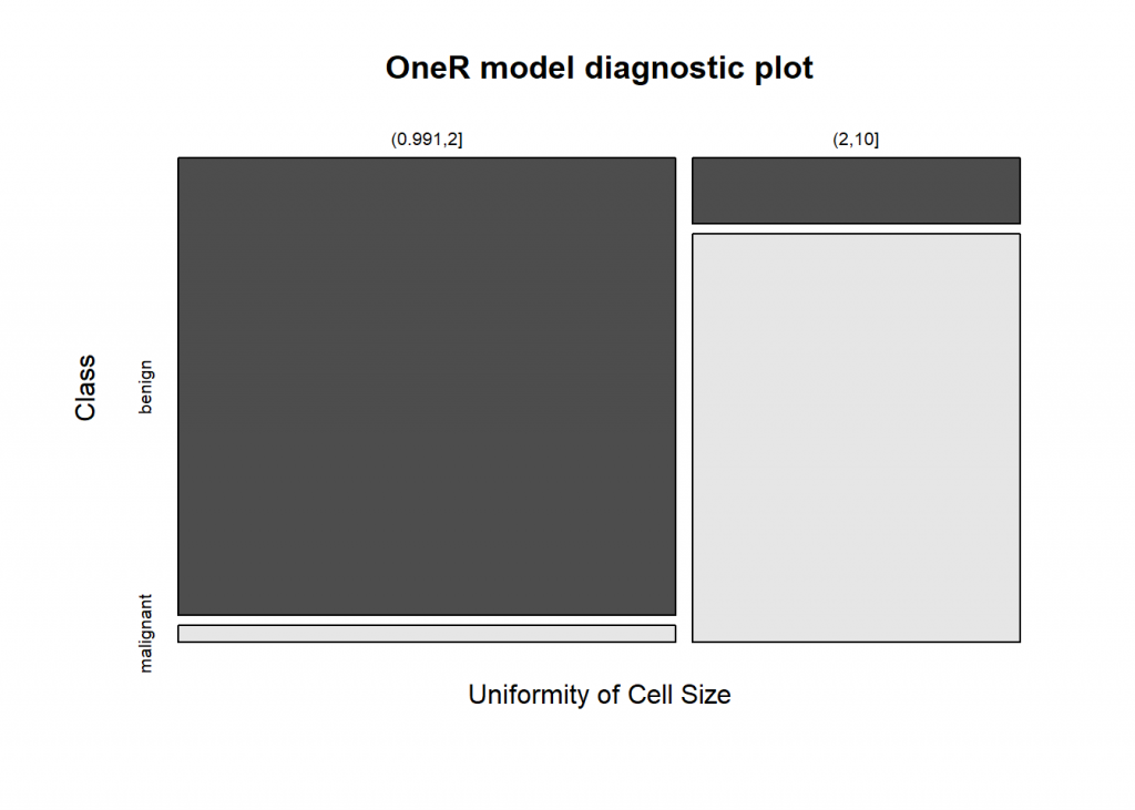
data(breastcancer)
data <- breastcancer

# Divide training (80%) and test set (20%)
set.seed(12) # for reproducibility
random <- sample(1:nrow(data), 0.8 * nrow(data))
data_train <- optbin(data[random, ], method = "infogain")
## Warning in optbin.data.frame(data[random, ], method = "infogain"): 12
## instance(s) removed due to missing values
data_test <- data[-random, ]

# Train OneR model on training set
model_train <- OneR(data_train, verbose = TRUE)
##
##     Attribute                   Accuracy
## 1 * Uniformity of Cell Size     92.32%
## 2   Uniformity of Cell Shape    91.59%
## 3   Bare Nuclei                 90.68%
## 4   Bland Chromatin             90.31%
## 5   Normal Nucleoli             90.13%
## 6   Single Epithelial Cell Size 89.4%
## 7   Marginal Adhesion           85.92%
## 8   Clump Thickness             84.28%
## 9   Mitoses                     78.24%
## ---
## Chosen attribute due to accuracy
## and ties method (if applicable): '*'

# Show model and diagnostics
summary(model_train)
##
## Call:
## OneR.data.frame(x = data_train, verbose = TRUE)
##
## Rules:
## If Uniformity of Cell Size = (0.991,2] then Class = benign
## If Uniformity of Cell Size = (2,10]    then Class = malignant
##
## Accuracy:
## 505 of 547 instances classified correctly (92.32%)
##
## Contingency table:
##            Uniformity of Cell Size
## Class       (0.991,2] (2,10] Sum
##   benign        * 318     30 348
##   malignant        12  * 187 199
##   Sum             330    217 547
## ---
## Maximum in each column: '*'
##
## Pearson's Chi-squared test:
## X-squared = 381.78243, df = 1, p-value < 0.00000000000000022204

# Plot model diagnostics
plot(model_train)
# Use trained model to predict test set
prediction <- predict(model_train, data_test)

# Evaluate model performance on test set
eval_model(prediction, data_test)
##
## Confusion matrix (absolute):
##            Actual
## Prediction  benign malignant Sum
##   benign        92         0  92
##   malignant      8        40  48
##   Sum          100        40 140
##
## Confusion matrix (relative):
##            Actual
## Prediction  benign malignant  Sum
##   benign      0.66      0.00 0.66
##   malignant   0.06      0.29 0.34
##   Sum         0.71      0.29 1.00
##
## Accuracy:
## 0.9429 (132/140)
##
## Error rate:
## 0.0571 (8/140)
##
## Error rate reduction (vs. base rate):
## 0.8 (p-value = 0.000000000007992571)
As you can see the accuracy is only slightly worse but you have full interpretability of the model… and you would only need to measure one value (“Uniformity of Cell Size”) instead of 9 to get a prediction!
On the other hand, making neural networks interpretable is one of the big research challenges at the moment. This area is called Explainable Artificial Intelligence or XAI and you can find out more here: Explainable AI (XAI)… Explained! Or: How to whiten any Black Box with LIME.
To end this rather long post: there is a real revolution going on at the moment with all kinds of powerful neural networks. Especially promising is a combination of reinforcement learning (the topic of an upcoming post) and neural networks, where the reinforcement learning algorithm uses a neural network as its memory. For example, the revolutionary AlphaGo Zero is built this way: it just received the rules of Go, one of the most demanding strategy games humanity has ever invented, and grew superhuman strength after just three days! The highest human rank in Go has an ELO value of 2940 – AlphaGo Zero achieves 5185! Even the best players don’t stand a chance against this monster of a machine. The neural network technology that is used for AlphaGo Zero and many other deep neural networks is called Tensorflow, which can also easily be integrated into the R environment. To find out more go here: https://tensorflow.rstudio.com/
In this whole area there are many mind-blowing projects underway, so stay tuned!
UPDATE June – October 2022
I created a video-series for this post (in German):
Wow, this was an amazing write-up. Very well structured, with code and real life applications. Super helpful. Looking forward to similar articles!
Dear Torsten, thank you very much for the great feedback… I really appreciate it! I have many more articles in the pipe, so stay tuned 🙂
A really great article with very clear and reproducible examples.
Thank you very much, Graham!
Great post, here. Thanks a lot for the simple enough examples as well.
Just one basic question … pardon me if this is really basic – but when you assign sample values to ‘weights’ – can we apply the human knowledge associated with say X1 or X2 to determine appropriate weights. For example, if i know as an SME that for a given population – clump thickness is more important than say uniformity of cell, and if i start giving that a 0.3 for clump thickness and 0.1 for say the other parameters, is that akin to saying that – am asking the machine to think like me ? as in the doctor who believes that for ‘this’ population, it is the thickness that matters more than others and so i make that decision. Kindly advise.
In many cases, i have noticed that the human brain has these ‘intuitions’ that seem to throw more weight on one dimension than the other and being new to Neural Network i wasn’t sure if we can follow the same here.
thanks once again.
Thank you for your great feedback!
I wouldn’t expect that this method of pre-assigning weights according to some domain knowledge would work: the reason is the same that we cannot understand the internal structure of bigger Neural Nets (a.k.a. black box problem). The knowledge of the net is not in the first few weights but in the intricate interaction of all neurons. Another thing is that with bigger nets you just have too many neurons that would need to be pre-assigned.
What does work though is what is called transfer learning: here you take a net that was trained for some similar task as the basis of your new net. I will talk about that in an upcoming post, so stay tuned!
Adding to my previous comment:
You sometimes can use domain knowledge for the topology of the net, data scientist Andriy Burkov from Gartner correctly asserts: “The designer of the convolutional NN for image classification has looked into the input data (this is what traditional ML engineers do to invent features) and decided that patches of pixels close to each other contain information that could help in classification, and at the same time reduce the number of NN parameters.”
Thank you … appreciate the immediate response.
Brings me to a follow up question … hope you don’t mind; question is – does it mean if the “black box” has a mind of its own and computes it’s own weights, could we then as humans look at that and validate our intuition ?
Or in other words, the corollary – i.e., if the weights coming through the NN are not in line with what the human mind goes by, then either – the human mind is inaccurate or we haven’t given enough data points to justify the weights as we think they should be. Would that be a fair statement? Do let us know what you think.
thanks once again. really appreciate the dialogue.
Can you explain in a little more details as to how the multi-layers extract different levels of abstraction from the images. How does it know that the first layers is for extraction of edges, then detection of elements of faces, like eyes and noses, and finally abstractions of certain faces. The network is simply assigning weights and there is no explicit coding for the levels, what is the real secret or computation ?
Basically, the net does that automatically by itself through training… like in the first example where it organized itself to represent the three heroes of our little story. Similar effects happen when neural nets are trained for language translation: they develop some kind of proto-language no human is able to understand.
The real secret you ask: unfortunately we still don’t know enough to know for sure what kind of convoluted dynamics really happen inside artificial neural networks… that is the sobering truth!
Thanks for the reply, I am amazed that the working is a blackbox. The “organization” is just adjustments of weights, but how the different layers separate out the features remains a wonder. Yet your article remains one of the best.
Hi, I like this article. So to learn ANN I started to repeat your example and already at the very beginning, I got a problem. First I typed everything by myself then I just copied your codes
And I always had got this:
round(compute(neuralnetwork, qualities)$net.result)
           [,1] [,2] [,3] [,4] [,5] [,6] [,7]
wolf         NA   NA   NA   NA   NA   NA   NA
grannie      NA   NA   NA   NA   NA   NA   NA
woodcutter   NA   NA   NA   NA   NA   NA   NA
I feel really stupid to write this, but could you tell me what is wrong?
Thank you, Ewa, I appreciate it!
It is not your fault!
computewas deprecated and was replaced bypredict(which is the general standard in the R sphere)… so thank you for the heads-up!I will update the code and come back to you…
Thank you 🙂
Ok, so I updated the code… for some reason the
predictfunction doesn’t work here (anybody an idea why? – please comment!), which isn’t a problem because I wanted to illustrate what the net learned and this is already saved in theneuralnetworkobject.In the second (more sophisticated) example
predictworks fine.It seems to be a problem with exclude. Without this I can bind another row to data via
data2 <- rbind(data, MrX=c(0,0,1,0,1,0,NA,NA,NA,NA,NA,NA,NA))
round(predict(neuralnetwork, data2))
Thanks for your great blogs! I got some nice ideas for my own statistics lectures and will recommend your blogs to my students 🙂
I tried to understand:
exclude = c(1, 8, 15, 22, 26, 30, 34, 38, 42, 46),What are the numbers meaning here? How can I determine them in the real praxis?
This is the somewhat strange way of excluding bias neurons in the
neuralnetpackage. See also my question (and answer) here: https://stackoverflow.com/q/40633567/468305.I’m not getting the same answers as the code the required the OneR library. Before that everything is the same. I copied the code from the website, so a typing error is not the issue.
Could try your version and see if the results are the same?
Thank you.
Yes, the reason is that some time ago the random number generator of R was changed so that the old seed values now lead to different random numbers (and therefore the dataset is split into a trainings- and test-set differently which leads to slightly different results).