

Correlation and its associated challenges don’t lose their fascination: most people know that correlation doesn’t imply causation, not many people know that the opposite is also true (see: Causation doesn’t imply Correlation either) and some know that correlation can just be random (so-called spurious correlation).
If you want to learn about a paradoxical effect nearly nobody is aware of, where correlation between two uncorrelated random variables is introduced just by sampling, read on!
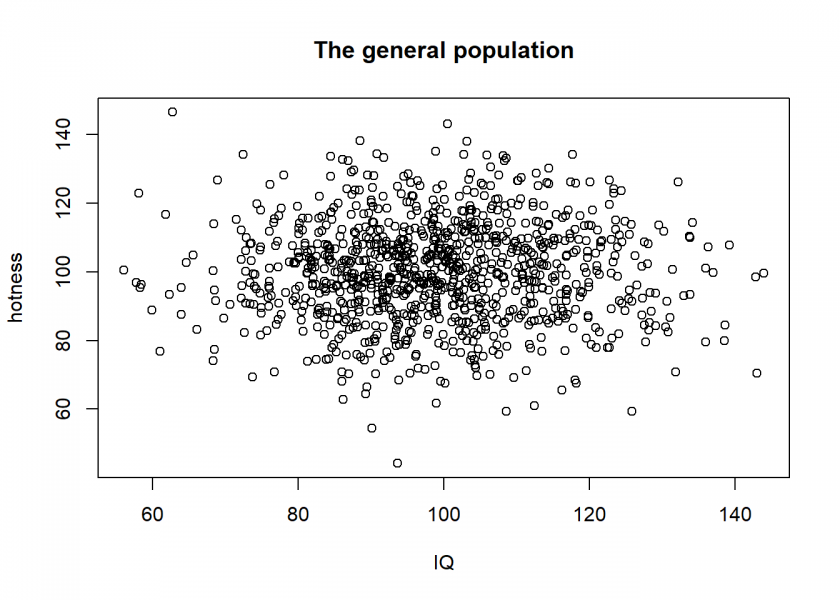
Let us just get into an example (inspired by When Correlation Is Not Causation, But Something Much More Screwy): for all intents and purposes let us assume that appearance and IQ are normally distributed and are uncorrelated:
set.seed(1147)
hotness <- rnorm(1000, 100, 15)
IQ <- rnorm(1000, 100, 15)
pop <- data.frame(hotness, IQ)
plot(hotness ~ IQ, main = "The general population")
Now, we can ask ourselves: why does somebody become famous? One plausible assumption (besides luck, see also: The Rich didn’t earn their Wealth, they just got Lucky) would be that this person has some combination of attributes. To stick with our example, let us assume some combination of hotness and intelligence and let us sample some “celebrities” on the basis of this combination:
pop$comb <- pop$hotness + pop$IQ # some combination of hotness and IQ

celebs <- pop[pop$comb > 235, ] # sample celebs on the basis of this combination
plot(celebs$hotness ~ celebs$IQ, xlab = "IQ", ylab = "hotness",  main = "Celebrities")
abline(lm(celebs$hotness ~ celebs$IQ), col = "red")
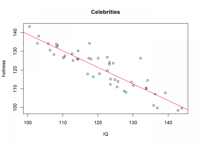
Wow, a clear negative relationship between hotness and IQ! Even a highly significant one (to understand significance, see also: From Coin Tosses to p-Hacking: Make Statistics Significant Again!):
cor.test(celebs$hotness, celebs$IQ) # highly significant
##
##  Pearson's product-moment correlation
##
## data:  celebs$hotness and celebs$IQ
## t = -14.161, df = 46, p-value < 2.2e-16
## alternative hypothesis: true correlation is not equal to 0
## 95 percent confidence interval:
##  -0.9440972 -0.8306163
## sample estimates:
##       cor
## -0.901897
How can this be? Well, the basis (the combination of hotness and IQ) on which we sample from our (uncorrelated) population is what is called a collider (variable) in statistics. Whereas a confounder (variable) influences (at least) two variables (A ← C → B), a collider is the opposite: it is influenced by (at least) two variables (A → C ← B).
In our simple case, it is the sum of our two independent variables, i.e. the variable “success” that could be considered the collider because it “collides” with the other variable and creates the bias.
The result is a spurious correlation introduced by a special form of selection bias, namely endogenous selection bias. The same effect also goes under the name Berkson’s paradox, Berkson’s fallacy, selection-distortion effect, conditioning on a collider (variable), collider stratification bias, or just collider bias.
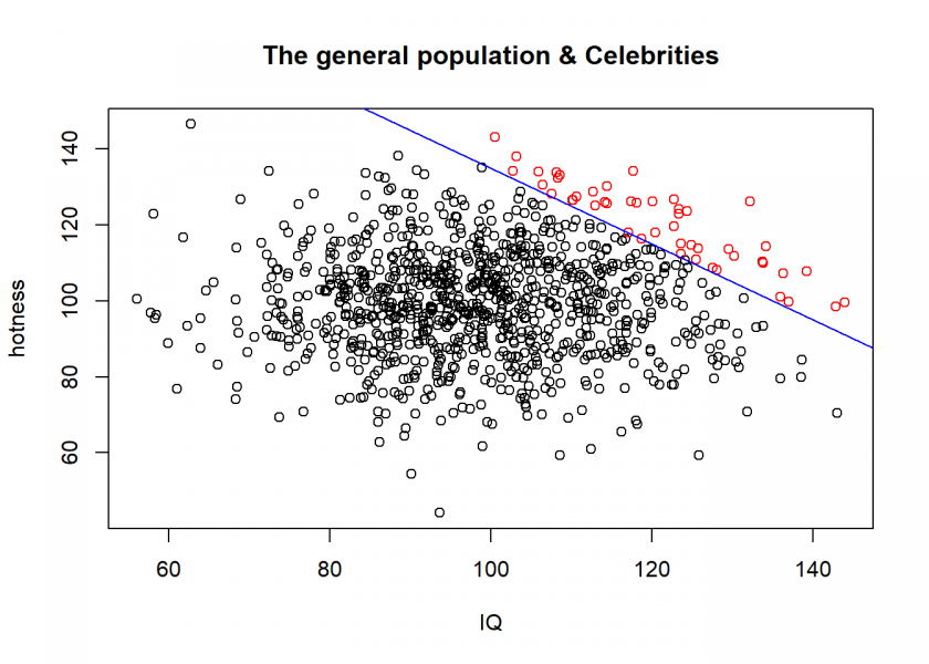
To understand this effect intuitively we are going to combine the two plots from above:
plot(hotness ~ IQ, main = "The general population & Celebrities")
points(celebs$hotness ~ celebs$IQ, col = "red")
abline(a = 235, b = -1, col = "blue")
In reality, things are often not so simple. When you google the above search terms you will find all kinds of examples, e.g. the so-called obesity paradox (an apparent preventive effect of obesity on mortality in individuals with cardiovascular disease (CVD)), a supposed health-protective effect of neuroticism or biased deep learning predictions of lung cancer.
As a takeaway: if a statistical result implies a relationship that seems too strange to be true, it possibly is! To check whether collider bias might be present check if sampling was being conducted on the basis of a variable that is influenced by the variables that seem to be correlated! Otherwise, you might not only falsely conclude that beautiful people are generally stupid and intelligent people ugly…
UPDATE February 2, 2023
I created a video for this post (in German):
The concept of “selection bias” is more well known to explain the negative correlation in the example. But the concept of “collider” requires understanding graph theory or Bayesian, which also can explain the negative correlation in the example.
So you just created an score to determine through the sum of two variables the relationship between two variables. How would you know if it is a collider in the middle or something related with collinearity?
Imagine I want to create a composite score using at least 5 variables, biomarkers in blood, how do I know if there is a collider?
Somehow it does scare me, beacause I see this quite often
Dear Javier, thank you for bringing up these important points, here is my reply:
Identifying a Collider: To determine if a composite score is a collider, you need to consider the causal relationships between the variables involved. If the score (or any variable for that matter) is influenced by two other variables in your study, and you also control for this score in your analysis, it could become a collider. This would bias the relationship between the variables that influence the score. Causal diagrams (DAGs – Directed Acyclic Graphs) are often used to identify potential colliders in a set of variables.
Dealing with Collinearity in Creating a Composite Score: When creating a composite score from multiple variables (e.g., biomarkers in blood), it’s crucial to check for collinearity among these variables. High collinearity can affect the stability and interpretation of the score. Techniques like checking the Variance Inflation Factor (VIF) can help assess the degree of collinearity. If collinearity is present, methods like Principal Component Analysis (PCA) or partial least squares regression might be used to reduce the dimensionality of the data while minimizing the impact of collinearity.
Practical Steps to Check for Colliders and Collinearity:
– Construct a Causal Model: Start by mapping out a causal model (using DAGs) of how you think the variables interact, which can help identify potential colliders.
– Analytical Checks for Collinearity: Use statistical methods to check for collinearity among the variables you plan to include in your composite score, such as calculating the correlation matrix or the Variance Inflation Factor (VIF).
– Model Testing: After creating your score, test the model for sensitivity to inclusion/exclusion of the composite score and observe any changes in the relationships between other variables.
In summary, addressing these issues involves a combination of careful design of the study, understanding the underlying causal relationships, and appropriate statistical analyses to detect and mitigate issues like collider bias and collinearity.