

As promised in the post Learning Data Science: Modelling Basics we will now go a step further and try to predict income brackets with real world data and different modelling approaches. We will learn a thing or two along the way, e.g. about the so-called Accuracy-Interpretability Trade-Off, so read on…
The data we will use is from here: Marketing data set. The description reads:
This dataset contains questions from questionnaires that were filled out by shopping mall customers in the San Francisco Bay area. The goal is to predict the Annual Income of Household from the other 13 demographics attributes.
The following extra information (or metadata) is provided with the data:
cat(readLines('data/marketing-names.txt'), sep = '\n')
Marketing data set
1: Description.
This dataset contains questions from questionaries that were filled out by shopping mall customers in the San Francisco Bay area. The goal is to predict the Annual Income of Household from the other 13 demographics attributes.
2: Type.            Classification
3: Origin.          Real world
4: Instances.       6876 (8993)
5: Features.        14
6: Classes          9
7: Missing values.  Yes
8: Header.
@relation marketing
@attribute Sex integer [1, 2]
@attribute MaritalStatus integer [1, 5]
@attribute Age integer [1, 7]
@attribute Education integer [1, 6]
@attribute Occupation integer [1, 9]
@attribute YearsInSf integer [1, 5]
@attribute DualIncome integer [1, 3]
@attribute HouseholdMembers integer [1, 9]
@attribute Under18 integer [0, 9]
@attribute HouseholdStatus integer [1, 3]
@attribute TypeOfHome integer [1, 5]
@attribute EthnicClass integer [1, 8]
@attribute Language integer [1, 3]
@attribute Income {1, 2, 3, 4, 5, 6, 7, 8, 9}
@inputs Sex, MaritalStatus, Age, Education, Occupation, YearsInSf, DualIncome, HouseholdMembers, Under18, HouseholdStatus, TypeOfHome, EthnicClass, Language
@outputs Income
DATA DICTIONARY
 1    ANNUAL INCOME OF HOUSEHOLD (PERSONAL INCOME IF SINGLE)
             1. Less than $10,000
             2. $10,000 to $14,999
             3. $15,000 to $19,999
             4. $20,000 to $24,999
             5. $25,000 to $29,999
             6. $30,000 to $39,999
             7. $40,000 to $49,999
             8. $50,000 to $74,999
             9. $75,000 or more

 2    SEX
             1. Male
             2. Female
  3    MARITAL STATUS
             1. Married
             2. Living together, not married
             3. Divorced or separated
             4. Widowed
             5. Single, never married
  4    AGE
             1. 14 thru 17
             2. 18 thru 24
             3. 25 thru 34
             4. 35 thru 44
             5. 45 thru 54
             6. 55 thru 64
             7. 65 and Over
  5    EDUCATION
             1. Grade 8 or less
             2. Grades 9 to 11
             3. Graduated high school
             4. 1 to 3 years of college
             5. College graduate
             6. Grad Study
 6    OCCUPATION
             1. Professional/Managerial
             2. Sales Worker
             3. Factory Worker/Laborer/Driver
             4. Clerical/Service Worker
             5. Homemaker
             6. Student, HS or College
             7. Military
             8. Retired
             9. Unemployed
  7    HOW LONG HAVE YOU LIVED IN THE SAN FRAN./OAKLAND/SAN JOSE AREA?
             1. Less than one year
             2. One to three years
             3. Four to six years
             4. Seven to ten years
             5. More than ten years
  8    DUAL INCOMES (IF MARRIED)
             1. Not Married
             2. Yes
             3. No
  9    PERSONS IN YOUR HOUSEHOLD
             1. One
             2. Two
             3. Three
             4. Four
             5. Five
             6. Six
             7. Seven
             8. Eight
             9. Nine or more

 10    PERSONS IN HOUSEHOLD UNDER 18
             0. None
             1. One
             2. Two
             3. Three
             4. Four
             5. Five
             6. Six
             7. Seven
             8. Eight
             9. Nine or more
 11    HOUSEHOLDER STATUS
             1. Own
             2. Rent
             3. Live with Parents/Family
 12    TYPE OF HOME
             1. House
             2. Condominium
             3. Apartment
             4. Mobile Home
             5. Other
 13    ETHNIC CLASSIFICATION
             1. American Indian
             2. Asian
             3. Black
             4. East Indian
             5. Hispanic
             6. Pacific Islander
             7. White
             8. Other
  14    WHAT LANGUAGE IS SPOKEN MOST OFTEN IN YOUR HOME?
             1. English
             2. Spanish
             3. Other
Our task is to predict the variable “Income”.
So, let us first load the data (you can find the correctly formatted csv-file here: marketing.csv), have a look at some of its characteristics and perform a little bit of additional formatting. After that we divide it into a training (80%) and a test set (20%) to account for potential overfitting (also see Learning Data Science: Modelling Basics):
data <- read.csv("data/marketing.csv") # change path accordingly
dim(data)
## [1] 6876   14

str(data)
## 'data.frame':    6876 obs. of  14 variables:
##  $ Sex             : int  1 2 2 2 1 1 1 1 1 1 ...
##  $ MaritalStatus   : int  1 1 5 5 1 5 3 1 1 5 ...
##  $ Age             : int  5 3 1 1 6 2 3 6 7 2 ...
##  $ Education       : int  5 5 2 2 4 3 4 3 4 4 ...
##  $ Occupation      : int  5 1 6 6 8 9 3 8 8 9 ...
##  $ YearsInSf       : int  5 5 5 3 5 4 5 5 4 5 ...
##  $ DualIncome      : int  3 2 1 1 3 1 1 3 3 1 ...
##  $ HouseholdMembers: int  5 3 4 4 2 3 1 3 2 1 ...
##  $ Under18         : int  2 1 2 2 0 1 0 0 0 0 ...
##  $ HouseholdStatus : int  1 2 3 3 1 2 2 2 2 2 ...
##  $ TypeOfHome      : int  1 3 1 1 1 3 3 3 3 3 ...
##  $ EthnicClass     : int  7 7 7 7 7 7 7 7 7 7 ...
##  $ Language        : int  1 1 1 1 1 1 1 1 1 1 ...
##  $ Income          : int  9 9 1 1 8 1 6 2 4 1 ...

data <- data.frame(data[-ncol(data)], Income = factor(data$Income))

set.seed(12)
random <- sample(1:nrow(data), 0.8 * nrow(data))
data_train <- data[random, ]
data_test <- data[-random, ]
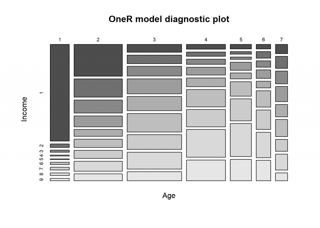
We start with a simple but comprehensible model, OneR (on CRAN), as a benchmark:
library(OneR)
data <- optbin(data_train)
model <- OneR(data, verbose = TRUE)
##
##     Attribute        Accuracy
## 1 * Age              28.2%
## 2   MaritalStatus    28.11%
## 3   Occupation       28.07%
## 4   HouseholdStatus  27.56%
## 5   DualIncome       27.04%
## 6   Education        25.98%
## 7   HouseholdMembers 22.51%
## 8   Under18          20.69%
## 9   TypeOfHome       19.36%
## 10  EthnicClass      19.29%
## 11  Sex              18.07%
## 12  Language         17.82%
## 13  YearsInSf        17.75%
## ---
## Chosen attribute due to accuracy
## and ties method (if applicable): '*'

summary(model)
##
## Call:
## OneR.data.frame(x = data, verbose = TRUE)
##
## Rules:
## If Age = 1 then Income = 1
## If Age = 2 then Income = 1
## If Age = 3 then Income = 6
## If Age = 4 then Income = 8
## If Age = 5 then Income = 8
## If Age = 6 then Income = 8
## If Age = 7 then Income = 6
##
## Accuracy:
## 1551 of 5500 instances classified correctly (28.2%)
##
## Contingency table:
##       Age
## Income     1     2     3     4     5    6    7  Sum
##    1   * 421 * 352    99    43    21   15   25  976
##    2      16   204   107    39    13   22   33  434
##    3       9   147   122    49    12   21   35  395
##    4       5   121   188    71    39   29   42  495
##    5       3    77   179    81    29   23   34  426
##    6      10    93 * 234   156    70   56 * 47  666
##    7      12    92   185   155   107   66   33  650
##    8      12   111   211 * 251 * 160 * 86   44  875
##    9      11    76   114   187   104   69   22  583
##    Sum   499  1273  1439  1032   555  387  315 5500
## ---
## Maximum in each column: '*'
##
## Pearson's Chi-squared test:
## X-squared = 2671.2, df = 48, p-value < 2.2e-16

plot(model)
prediction <- predict(model, data_test)
eval_model(prediction, data_test)
##
## Confusion matrix (absolute):
##           Actual
## Prediction    1    2    3    4    5    6    7    8    9  Sum
##        1    232   45   46   32   33   27   19   27   24  485
##        2      0    0    0    0    0    0    0    0    0    0
##        3      0    0    0    0    0    0    0    0    0    0
##        4      0    0    0    0    0    0    0    0    0    0
##        5      0    0    0    0    0    0    0    0    0    0
##        6     31   30   44   44   41   66   44   57   50  407
##        7      0    0    0    0    0    0    0    0    0    0
##        8     16   20   20   47   27   87   71  110   86  484
##        9      0    0    0    0    0    0    0    0    0    0
##        Sum  279   95  110  123  101  180  134  194  160 1376
##
## Confusion matrix (relative):
##           Actual
## Prediction    1    2    3    4    5    6    7    8    9  Sum
##        1   0.17 0.03 0.03 0.02 0.02 0.02 0.01 0.02 0.02 0.35
##        2   0.00 0.00 0.00 0.00 0.00 0.00 0.00 0.00 0.00 0.00
##        3   0.00 0.00 0.00 0.00 0.00 0.00 0.00 0.00 0.00 0.00
##        4   0.00 0.00 0.00 0.00 0.00 0.00 0.00 0.00 0.00 0.00
##        5   0.00 0.00 0.00 0.00 0.00 0.00 0.00 0.00 0.00 0.00
##        6   0.02 0.02 0.03 0.03 0.03 0.05 0.03 0.04 0.04 0.30
##        7   0.00 0.00 0.00 0.00 0.00 0.00 0.00 0.00 0.00 0.00
##        8   0.01 0.01 0.01 0.03 0.02 0.06 0.05 0.08 0.06 0.35
##        9   0.00 0.00 0.00 0.00 0.00 0.00 0.00 0.00 0.00 0.00
##        Sum 0.20 0.07 0.08 0.09 0.07 0.13 0.10 0.14 0.12 1.00
##
## Accuracy:
## 0.2965 (408/1376)
##
## Error rate:
## 0.7035 (968/1376)
##
## Error rate reduction (vs. base rate):
## 0.1176 (p-value < 2.2e-16)
What can we conclude from this? First, the most important feature is “Age” while “Marital Status”, “Occupation” and “Household Status” perform comparably well. The overall accuracy (i.e. the percentage of correctly predicted instances) is with about 30% not that great, on the other hand not that extraordinarily uncommon when dealing with real-world data. Looking at the model itself, in the form of rules and the diagnostic plot, we can see that we have non-linear relationship between Age and Income: the older one gets the higher the income bracket, except for people who are old enough to retire. This seems plausible.
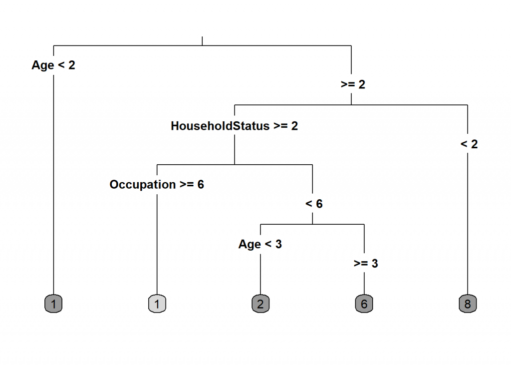
OneR is basically a one step decision tree, so the natural choice for our next analysis would be to have a full decision tree built (all packages are on CRAN):
library(rpart)
library(rpart.plot)
model <- rpart(Income ~., data = data_train)
rpart.plot(model, type = 3, extra = 0, box.palette = "Grays")
prediction <- predict(model, data_test, type = "class")
eval_model(prediction, data_test)
##
## Confusion matrix (absolute):
##           Actual
## Prediction    1    2    3    4    5    6    7    8    9  Sum
##        1    201   36   22   13   16   12    8   15   12  335
##        2     43   25   32   22   17   12   10   14    6  181
##        3      0    0    0    0    0    0    0    0    0    0
##        4      0    0    0    0    0    0    0    0    0    0
##        5      0    0    0    0    0    0    0    0    0    0
##        6     18   24   40   50   42   68   32   33   22  329
##        7      0    0    0    0    0    0    0    0    0    0
##        8     17   10   16   38   26   88   84  132  120  531
##        9      0    0    0    0    0    0    0    0    0    0
##        Sum  279   95  110  123  101  180  134  194  160 1376
##
## Confusion matrix (relative):
##           Actual
## Prediction    1    2    3    4    5    6    7    8    9  Sum
##        1   0.15 0.03 0.02 0.01 0.01 0.01 0.01 0.01 0.01 0.24
##        2   0.03 0.02 0.02 0.02 0.01 0.01 0.01 0.01 0.00 0.13
##        3   0.00 0.00 0.00 0.00 0.00 0.00 0.00 0.00 0.00 0.00
##        4   0.00 0.00 0.00 0.00 0.00 0.00 0.00 0.00 0.00 0.00
##        5   0.00 0.00 0.00 0.00 0.00 0.00 0.00 0.00 0.00 0.00
##        6   0.01 0.02 0.03 0.04 0.03 0.05 0.02 0.02 0.02 0.24
##        7   0.00 0.00 0.00 0.00 0.00 0.00 0.00 0.00 0.00 0.00
##        8   0.01 0.01 0.01 0.03 0.02 0.06 0.06 0.10 0.09 0.39
##        9   0.00 0.00 0.00 0.00 0.00 0.00 0.00 0.00 0.00 0.00
##        Sum 0.20 0.07 0.08 0.09 0.07 0.13 0.10 0.14 0.12 1.00
##
## Accuracy:
## 0.3096 (426/1376)
##
## Error rate:
## 0.6904 (950/1376)
##
## Error rate reduction (vs. base rate):
## 0.134 (p-value < 2.2e-16)
The new model has an accuracy that is a little bit better but the interpretability is a little bit worse. You have to go through the different branches to see in which income bracket it ends. So, for example, when the age bracket is below  (which means that it is
  ) it predicts income bracket when it is bigger than and the Household Status bracket is it predicts income bracket
  and so on. The most important variable, as you can see is again Age (which is reassuring that OneR was on the right track) but we also see Household Status and Occupation again.
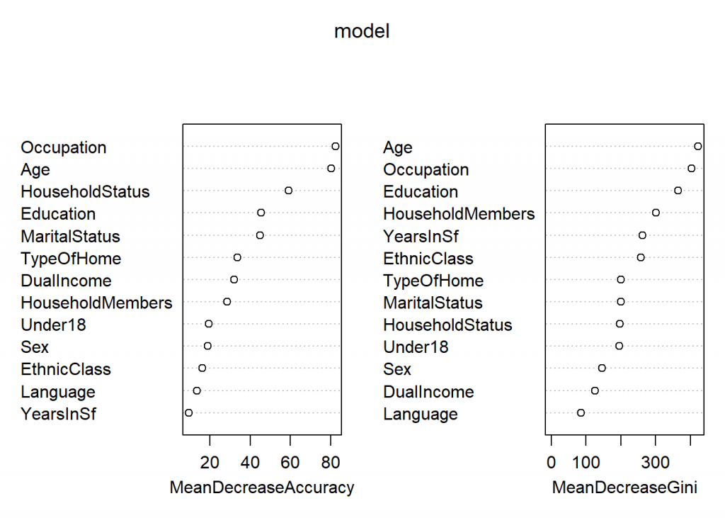
What is better than one tree? Many trees! So the next natural step is to have many trees built while varying the features and the examples that should be included in each tree. In the end it may be that different trees give different income brackets as their respective predictions, which we solve via voting as in a good democracy. This whole method is fittingly called Random Forests and fortunately there are many good packages available in R. We use the randomForest package (also on CRAN) here:
library(randomForest)
## randomForest 4.6-14
## Type rfNews() to see new features/changes/bug fixes.

set.seed(4543) # for reproducibility
model <- randomForest(Income ~., data = data_train, importance = TRUE)
varImpPlot(model)
prediction <- predict(model, data_test)
eval_model(prediction, data_test)
##
## Confusion matrix (absolute):
##           Actual
## Prediction    1    2    3    4    5    6    7    8    9  Sum
##        1    223   35   26   16   19   11    9   18   16  373
##        2     24   15   12   20    7   11    1    4    1   95
##        3      9   10   11   14    9    6    3    4    2   68
##        4      5   15   25   22   10   22    6    9    5  119
##        5      2    2    8    9    6   12    6    3    1   49
##        6      3    5   15   14   19   40   23   17   15  151
##        7      8    4    7   13   14   26   25   24    5  126
##        8      3    8    5   11   13   44   49   87   68  288
##        9      2    1    1    4    4    8   12   28   47  107
##        Sum  279   95  110  123  101  180  134  194  160 1376
##
## Confusion matrix (relative):
##           Actual
## Prediction    1    2    3    4    5    6    7    8    9  Sum
##        1   0.16 0.03 0.02 0.01 0.01 0.01 0.01 0.01 0.01 0.27
##        2   0.02 0.01 0.01 0.01 0.01 0.01 0.00 0.00 0.00 0.07
##        3   0.01 0.01 0.01 0.01 0.01 0.00 0.00 0.00 0.00 0.05
##        4   0.00 0.01 0.02 0.02 0.01 0.02 0.00 0.01 0.00 0.09
##        5   0.00 0.00 0.01 0.01 0.00 0.01 0.00 0.00 0.00 0.04
##        6   0.00 0.00 0.01 0.01 0.01 0.03 0.02 0.01 0.01 0.11
##        7   0.01 0.00 0.01 0.01 0.01 0.02 0.02 0.02 0.00 0.09
##        8   0.00 0.01 0.00 0.01 0.01 0.03 0.04 0.06 0.05 0.21
##        9   0.00 0.00 0.00 0.00 0.00 0.01 0.01 0.02 0.03 0.08
##        Sum 0.20 0.07 0.08 0.09 0.07 0.13 0.10 0.14 0.12 1.00
##
## Accuracy:
## 0.3459 (476/1376)
##
## Error rate:
## 0.6541 (900/1376)
##
## Error rate reduction (vs. base rate):
## 0.1796 (p-value < 2.2e-16)
As an aside you can see that the basic modelling workflow stayed the same – no matter what approach (OneR, decision tree or random forest) you chose. This standard is kept for most (modern) packages and one of the great strengths of R! With thousands of packages on CRAN alone there are of course sometimes differences but those are normally well documented (so the help function or the vignette are your friends!)
Now, back to the result of the last analysis: again, the overall accuracy is better but because we have hundreds of trees now the interpretability suffered a lot. This is also known under the name Accuracy-Interpretability Trade-Off. The best we can do in the case of random forests is to find out which features are the most important ones. Again Age, Occupation and Household Status show up, which is consistent with our analyses so far. Additionally, because of the many trees that had to be built, this analysis ran a lot longer than the other two.
The following table shows those trade-offs for OneR, decision trees, random forests and neural networks (deep learning):

Random forests are one of the best methods out of the box, so the accuracy of about 34% tells us that our first model (OneR) wasn’t doing too bad in the first place! Why are able to reach comparatively good results with just one feature. This is true for many real-world data sets. Sometimes simple models are not much worse than very complicated ones – you should keep that in mind!
If you play around with this dataset I would be interested in your results! Please post them in the comments – Thank you and stay tuned!
UPDATE April 16, 2023
I created a video for this post (in German):
Very nice.
Thank you !!!
Thank you, much appreciated!
Hi
Looks interesting.
When I do this:
data <- read.csv("data/marketing.dat")I get the error:
Best,
Peter
Good point, thank you for the heads-up! I uploaded the correctly formatted csv-file to my server: marketing.csv)
You will have to change “dat” to “csv” – hope this helps
(Also edited the post accordingly)
Holger – thanks for yet another
clear, excellent post.
quick Q:
——
the RandomForest plot
shows 2 plots side-by-side:
* Accuracy and
* Gini.
Which plot should we use
to determine Var importance?.
In simple terms,
what is the difference btw these 2 plots?.
Thanks / Danke!
Ray
SF
Thank you for your question. You can find an excellent discussion on Stats.SE: How to interpret Mean Decrease in Accuracy and Mean Decrease GINI in Random Forest models.
Thank you for the helpful blogs.
when I run:
then got the warning:
Warnmeldung:
Thank you for your great feedback, highly appreciated.
As stated in the documentation: “If data contains unused factor levels (e.g. due to subsetting) these are ignored and a warning is given.”
Hi, thanks for your blogs and all the work, super excited with getting into R programming easily!
just a quick Q:
when I run:
thanks in advance!
best Oli
Dear olivier: Thank you for feedback!
I unfortunately cannot reproduce your error. Have you run
data <- read.csv("data/marketing.csv") # change path accordingly
dim(data)
str(data)
data <- data.frame(data[-ncol(data)], Income = factor(data$Income))

set.seed(12)
random <- sample(1:nrow(data), 0.8 * nrow(data))
before that and does it give you the same results as in the text (i.e. that the dataset was loaded correctly)?
best,
h