

In one of my most popular posts So, what is AI really? I showed that Artificial Intelligence (AI) basically boils down to autonomously learned rules, i.e. conditional statements or simply, conditionals.
In this post, I create the simplest possible classifier, called ZeroR, to show that even this classifier can achieve surprisingly high values for accuracy (i.e. the ratio of correctly predicted instances)… and why this is not necessarily a good thing, so read on!
In the above-mentioned post, I gave an example of a classifier that was able to give you some guidance on whether a certain mushroom is edible or not. The basis for this was rules, which separated the examples based on the given attributes:
## Rules:
## If odor = almond   then type = edible
## If odor = anise    then type = edible
## If odor = creosote then type = poisonous
## If odor = fishy    then type = poisonous
## If odor = foul     then type = poisonous
## If odor = musty    then type = poisonous
## If odor = none     then type = edible
## If odor = pungent  then type = poisonous
## If odor = spicy    then type = poisonous
Obviously, the more rules the more complex a classifier is. In the example above we used the so-called OneR classifier which bases its decision on one attribute alone. Here, I will give you an even simpler classifier! The ZeroR classifier bases its decision on no attribute whatsoever… zero, zilch, zip, nada! How can this be? Easy: it just takes the majority class of the target attribute! I will give you an example.
First, we build a function for the classifier by using the OneR package (on CRAN) and some S3-class magic:
library(OneR)

ZeroR <- function(x, ...) {
  output <- OneR(cbind(dummy = TRUE, x[ncol(x)]), ...)
  class(output) <- c("ZeroR", "OneR")
  output
}
predict.ZeroR <- function(object, newdata, ...) {
  class(object) <- "OneR"
  predict(object, cbind(dummy = TRUE, newdata[ncol(newdata)]), ...)
}
As an example we take the well-known German Credit Dataset (originally from my old alma mater, the University of Hamburg) and divide it into a training and a test set:
data <- read.table("data/german.data", header = FALSE)
data <- data.frame(data[ , 1:20], creditrisk = factor(data[ , 21]))
table(data$creditrisk)
##
##   1   2
## 700 300

set.seed(805)
random <- sample(1:nrow(data), 0.6 * nrow(data))
data_train <- data[random, ]
data_test <- data[-random, ]
We see that 700 customers have a good credit risk while 300 have a bad one. The ZeroR classifier now takes the majority class (good credit risk) and uses it as the prediction every time! You have read correctly, it just predicts that every customer is a good credit risk!
Seems a little crazy, right? Well, it illustrates an important point: many of my students, as well as some of my consulting clients, often ask me what a good classifier is and how long it does take to build one. Many people in the area of data science (even some “experts”) will give you something like the following answer (source: A. Burkov):
Machine learning accuracy rule:
0-80%: one day
80-90%: one week
90-95%: one month
95-97%: three months
97-99%: one year (or never)
Well, to be honest with you: this is not a very good answer. Why? Because it very much depends on… the share of the majority class! To understand that, let us have a look at how the ZeroR classifier performs on our dataset:
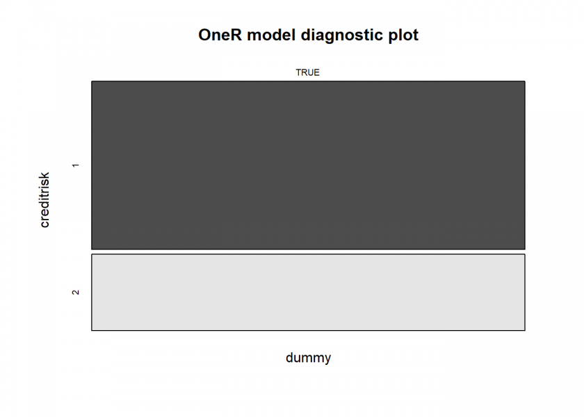
model <- ZeroR(data_train)
summary(model)
##
## Call:
## OneR.data.frame(x = cbind(dummy = TRUE, x[ncol(x)]))
##
## Rules:
## If dummy = TRUE then creditrisk = 1
##
## Accuracy:
## 481 of 700 instances classified correctly (68.71%)
##
## Contingency table:
##           dummy
## creditrisk  TRUE Sum
##        1   * 481 481
##        2     219 219
##        Sum   700 700
## ---
## Maximum in each column: '*'
##
## Pearson's Chi-squared test:
## X-squared = 98.063, df = 1, p-value < 2.2e-16

plot(model)
prediction <- predict(model, data_test)
eval_model(prediction, data_test)
##
## Confusion matrix (absolute):
##           Actual
## Prediction   1   2 Sum
##        1   219  81 300
##        2     0   0   0
##        Sum 219  81 300
##
## Confusion matrix (relative):
##           Actual
## Prediction    1    2  Sum
##        1   0.73 0.27 1.00
##        2   0.00 0.00 0.00
##        Sum 0.73 0.27 1.00
##
## Accuracy:
## 0.73 (219/300)
##
## Error rate:
## 0.27 (81/300)
##
## Error rate reduction (vs. base rate):
## 0 (p-value = 0.5299)
So, because 70% of the customers are good risks we get an accuracy of about 70%! You can take this example to extremes: for example, if you have a dataset with credit card transactions where 0.1% of the transactions are fraudulent (which is about the actual number) you will get an accuracy of 99.9% just by using the ZeroR classifier! Concretely, just by saying that no fraud exists (!) you get an accuracy even beyond the “one year (or never)” bracket (according to the above scheme)!
Another example even concerns life and death: the probability of dying within one year lies at about 0.8% (averaged over all the people worldwide, according to “The World Factbook” by the CIA). So by declaring that we are all immortal, we are in more than 99% of all cases right! Many medical studies have a much higher error rate… 😉
Now, let us try the OneR classifier on our credit dataset:
model <- OneR(optbin(data_train))
summary(model)
##
## Call:
## OneR.data.frame(x = optbin(data_train))
##
## Rules:
## If V3 = A30 then creditrisk = 2
## If V3 = A31 then creditrisk = 2
## If V3 = A32 then creditrisk = 1
## If V3 = A33 then creditrisk = 1
## If V3 = A34 then creditrisk = 1
##
## Accuracy:
## 492 of 700 instances classified correctly (70.29%)
##
## Contingency table:
##           V3
## creditrisk  A30  A31   A32  A33   A34 Sum
##        1     10   14 * 247 * 37 * 173 481
##        2   * 16 * 19   124   21    39 219
##        Sum   26   33   371   58   212 700
## ---
## Maximum in each column: '*'
##
## Pearson's Chi-squared test:
## X-squared = 39.504, df = 4, p-value = 5.48e-08

plot(model)
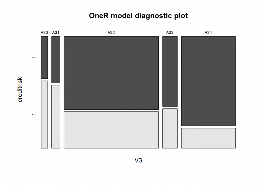
# Attribute 3:  (qualitative)
# Credit history
# A30 : no credits taken/
#   all credits paid back duly
# A31 : all credits at this bank paid back duly
# A32 : existing credits paid back duly till now
# A33 : delay in paying off in the past
# A34 : critical account/
#   other credits existing (not at this bank)

prediction <- predict(model, data_test)
eval_model(prediction, data_test)
##
## Confusion matrix (absolute):
##           Actual
## Prediction   1   2 Sum
##        1   207  63 270
##        2    12  18  30
##        Sum 219  81 300
##
## Confusion matrix (relative):
##           Actual
## Prediction    1    2  Sum
##        1   0.69 0.21 0.90
##        2   0.04 0.06 0.10
##        Sum 0.73 0.27 1.00
##
## Accuracy:
## 0.75 (225/300)
##
## Error rate:
## 0.25 (75/300)
##
## Error rate reduction (vs. base rate):
## 0.0741 (p-value = 0.2388)
Here, we see that we get an out-of-sample accuracy of 75%, which is more than 7 percentage points better than what we got with the ZeroR classifier, here called base rate. Yet, this is not statistically significant (for an introduction to statistical significance see From Coin Tosses to p-Hacking: Make Statistics Significant Again!).
Because the concept of “error rate reduction” compared to ZeroR (= base rate) and its statistical significance is so relevant it is displayed by default in the eval_model() function of the OneR package.
To end this post, we build a random forest model with the randomForest package (on CRAN) on the dataset (for some more information on random forests see Learning Data Science: Predicting Income Brackets):
set.seed(78)
library(randomForest)
## randomForest 4.6-14
## Type rfNews() to see new features/changes/bug fixes.

model <- randomForest(creditrisk ~., data = data_train, ntree = 2000)
prediction <- predict(model, data_test)
eval_model(prediction, data_test)
##
## Confusion matrix (absolute):
##           Actual
## Prediction   1   2 Sum
##        1   209  43 252
##        2    10  38  48
##        Sum 219  81 300
##
## Confusion matrix (relative):
##           Actual
## Prediction    1    2  Sum
##        1   0.70 0.14 0.84
##        2   0.03 0.13 0.16
##        Sum 0.73 0.27 1.00
##
## Accuracy:
## 0.8233 (247/300)
##
## Error rate:
## 0.1767 (53/300)
##
## Error rate reduction (vs. base rate):
## 0.3457 (p-value = 9.895e-05)
The out-of-sample accuracy is over 80% here and the error rate reduction (compared to ZeroR) of about one third is statistically significant. Yet 80% is still not that impressive when you keep in mind that 70% is the base rate!
You should now be able to spot why this is one of the worst scientific papers I have ever seen: Applications of rule based Classification Techniques for Thoracic Surgery (2015). This also shows one of the more general problems: although this is a medical topic not many medical professionals would be able to spot the elephant in the room here… this will be true for most other areas too, where machine learning will be used ever more frequently. (Just as an aside: this type of blunder wouldn’t have happened had the authors used the OneR package: One Rule (OneR) Machine Learning Classification in under One Minute.)
As you can imagine, there are many strategies to deal with the above challenges of imbalanced/unbalanced data, e.g. other model metrics (like recall or precision) and other sampling strategies (like undersampling the majority class or oversampling the minority class)… but that are topics for another post, so stay tuned!
Hi. I need your help with this new algorithm that you proposed. I have very short time please get back to me today.
Also, is there a research paper on Zeror classifier? If so, please provide link.
Please get back to me soon.
What exactly do you need? No, because it is so basic I don’t know any research paper on the ZeroR classifier?