

A few months ago, I posted about market basket analysis (see Customers who bought…), in this post we will see another form of it, done with Logistic Regression, so read on…
A big supermarket chain wanted to target (wink, wink) certain customer groups better. In this special case we are talking about pregnant women. The story goes that they identified a young girl as being pregnant and kept sending her coupons for baby care products. Now, the father got angry because she was “too young”… and complained to the supermarket. The whole story took a turn when his daughter confessed that… well, you know what! We are now going to reproduce a similar model here!
In this example, we have a dataset with products bought by customers with the additional information whether the respective buyer was pregnant or not. This is coded in the last column as 1 for pregnant and 0 for not pregnant, 500 instances each. As always, all kinds of analyses could be used but we stick with good old logistic regression because, first, it works quite well, and second, as we will see, the results are interpretable in this case.
Have a look at the following code (the data is from the book “Data Smart” by John Foreman: ch06.zip, save it, extract it, open it in Excel, delete the empty column before the last column PREGNANT and save the first sheet as a csv-file):
RetailMart <- read.csv("data/RetailMart.csv") # change path accordingly, you might have to use read.csv2 depending on your country version of Excel

head(RetailMart)
##   Implied.Gender Home.Apt..PO.Box Pregnancy.Test Birth.Control Feminine.Hygiene
## 1              M                A              1             0                0
## 2              M                H              1             0                0
## 3              M                H              1             0                0
## 4              U                H              0             0                0
## 5              F                A              0             0                0
## 6              F                H              0             0                0
##   Folic.Acid Prenatal.Vitamins Prenatal.Yoga Body.Pillow Ginger.Ale Sea.Bands
## 1          0                 1             0           0          0         0
## 2          0                 1             0           0          0         0
## 3          0                 0             0           0          0         1
## 4          0                 0             0           0          1         0
## 5          0                 0             1           0          0         0
## 6          0                 1             0           0          0         0
##   Stopped.buying.ciggies Cigarettes Smoking.Cessation Stopped.buying.wine Wine
## 1                      0          0                 0                   0    0
## 2                      0          0                 0                   0    0
## 3                      0          0                 0                   0    0
## 4                      0          0                 0                   0    0
## 5                      0          0                 0                   1    0
## 6                      1          0                 0                   0    0
##   Maternity.Clothes PREGNANT
## 1                 0        1
## 2                 0        1
## 3                 0        1
## 4                 0        1
## 5                 0        1
## 6                 0        1

tail(RetailMart)
##      Implied.Gender Home.Apt..PO.Box Pregnancy.Test Birth.Control
## 995               M                H              0             0
## 996               M                A              0             0
## 997               F                A              0             0
## 998               M                H              0             0
## 999               U                H              0             0
## 1000              M                A              0             0
##      Feminine.Hygiene Folic.Acid Prenatal.Vitamins Prenatal.Yoga Body.Pillow
## 995                 1          0                 0             0           0
## 996                 0          0                 0             0           0
## 997                 0          0                 0             0           0
## 998                 1          0                 0             0           0
## 999                 0          0                 0             0           0
## 1000                0          0                 0             0           0
##      Ginger.Ale Sea.Bands Stopped.buying.ciggies Cigarettes Smoking.Cessation
## 995           0         1                      0          0                 0
## 996           0         0                      0          0                 0
## 997           0         0                      0          0                 0
## 998           0         0                      0          0                 0
## 999           0         0                      0          0                 0
## 1000          1         0                      0          0                 0
##      Stopped.buying.wine Wine Maternity.Clothes PREGNANT
## 995                    0    0                 0        0
## 996                    0    0                 0        0
## 997                    0    0                 0        0
## 998                    0    0                 0        0
## 999                    0    0                 0        0
## 1000                   0    0                 1        0

table(RetailMart$PREGNANT)
##
##   0   1
## 500 500

str(RetailMart)
## 'data.frame':    1000 obs. of  18 variables:
##  $ Implied.Gender        : chr  "M" "M" "M" "U" ...
##  $ Home.Apt..PO.Box      : chr  "A" "H" "H" "H" ...
##  $ Pregnancy.Test        : int  1 1 1 0 0 0 0 0 0 0 ...
##  $ Birth.Control         : int  0 0 0 0 0 0 1 0 0 0 ...
##  $ Feminine.Hygiene      : int  0 0 0 0 0 0 0 0 0 0 ...
##  $ Folic.Acid            : int  0 0 0 0 0 0 1 0 0 0 ...
##  $ Prenatal.Vitamins     : int  1 1 0 0 0 1 1 0 0 1 ...
##  $ Prenatal.Yoga         : int  0 0 0 0 1 0 0 0 0 0 ...
##  $ Body.Pillow           : int  0 0 0 0 0 0 0 0 0 0 ...
##  $ Ginger.Ale            : int  0 0 0 1 0 0 0 0 1 0 ...
##  $ Sea.Bands             : int  0 0 1 0 0 0 0 0 0 0 ...
##  $ Stopped.buying.ciggies: int  0 0 0 0 0 1 0 0 0 0 ...
##  $ Cigarettes            : int  0 0 0 0 0 0 0 0 0 0 ...
##  $ Smoking.Cessation     : int  0 0 0 0 0 0 0 0 0 0 ...
##  $ Stopped.buying.wine   : int  0 0 0 0 1 0 0 0 0 0 ...
##  $ Wine                  : int  0 0 0 0 0 0 0 0 0 0 ...
##  $ Maternity.Clothes     : int  0 0 0 0 0 0 0 1 0 1 ...
##  $ PREGNANT              : int  1 1 1 1 1 1 1 1 1 1 ...
The metadata for each feature are the following:
- Account holder is Male/Female/Unknown by matching surname to census data.
- Account holder address is a home, apartment, or PO box.
- Recently purchased a pregnancy test
- Recently purchased birth control
- Recently purchased feminine hygiene products
- Recently purchased folic acid supplements
- Recently purchased prenatal vitamins
- Recently purchased prenatal yoga DVD
- Recently purchased body pillow
- Recently purchased ginger ale
- Recently purchased Sea-Bands
- Bought cigarettes regularly until recently, then stopped
- Recently purchased cigarettes
- Recently purchased smoking cessation products (gum, patch, etc.)
- Bought wine regularly until recently, then stopped
- Recently purchased wine
- Recently purchased maternity clothing
For building the actual model we use glm (for generalized linear model):
logreg <- glm(PREGNANT ~ ., data = RetailMart, family = binomial) # logistic regression - glm stands for generalized linear model
summary(logreg)
##
## Call:
## glm(formula = PREGNANT ~ ., family = binomial, data = RetailMart)
##
## Deviance Residuals:
##     Min       1Q   Median       3Q      Max
## -3.2012  -0.5566  -0.0246   0.5127   2.8658
##
## Coefficients:
##                         Estimate Std. Error z value Pr(>|z|)
## (Intercept)            -0.343597   0.180755  -1.901 0.057315 .
## Implied.GenderM        -0.453880   0.197566  -2.297 0.021599 *
## Implied.GenderU         0.141939   0.307588   0.461 0.644469
## Home.Apt..PO.BoxH      -0.172927   0.194591  -0.889 0.374180
## Home.Apt..PO.BoxP      -0.002813   0.336432  -0.008 0.993329
## Pregnancy.Test          2.370554   0.521781   4.543 5.54e-06 ***
## Birth.Control          -2.300272   0.365270  -6.297 3.03e-10 ***
## Feminine.Hygiene       -2.028558   0.342398  -5.925 3.13e-09 ***
## Folic.Acid              4.077666   0.761888   5.352 8.70e-08 ***
## Prenatal.Vitamins       2.479469   0.369063   6.718 1.84e-11 ***
## Prenatal.Yoga           2.922974   1.146990   2.548 0.010822 *
## Body.Pillow             1.261037   0.860617   1.465 0.142847
## Ginger.Ale              1.938502   0.426733   4.543 5.55e-06 ***
## Sea.Bands               1.107530   0.673435   1.645 0.100053
## Stopped.buying.ciggies  1.302222   0.342347   3.804 0.000142 ***
## Cigarettes             -1.443022   0.370120  -3.899 9.67e-05 ***
## Smoking.Cessation       1.790779   0.512610   3.493 0.000477 ***
## Stopped.buying.wine     1.383888   0.305883   4.524 6.06e-06 ***
## Wine                   -1.565539   0.348910  -4.487 7.23e-06 ***
## Maternity.Clothes       2.078202   0.329432   6.308 2.82e-10 ***
## ---
## Signif. codes:  0 '***' 0.001 '**' 0.01 '*' 0.05 '.' 0.1 ' ' 1
##
## (Dispersion parameter for binomial family taken to be 1)
##
##     Null deviance: 1386.29  on 999  degrees of freedom
## Residual deviance:  744.11  on 980  degrees of freedom
## AIC: 784.11
##
## Number of Fisher Scoring iterations: 7
Concerning interpretability, have a look at the output of the summary function above. First, you can see that some features have more stars than others. This has to do with their statistical significance (see also here: From Coin Tosses to p-Hacking: Make Statistics Significant Again!) and hints at whether the respective feature has some real influence on the outcome and is not just some random noise. We see that e.g., Pregnancy.Test, Birth.Control and Folic.Acid but also alcohol- and cigarette-related features get the maximum of three stars and are therefore considered highly significant for the model.
Another value is the estimate given for each feature which shows how strongly each feature influences the final model (because all feature values are normalized to being either 0 or 1) and in which direction. We can e.g., see that buying pregnancy tests and quitting smoking are quite strong predictors for being pregnant (no surprises here). An interesting case is the sex of the customers: both are not statistically significant, and both point in the same direction. The answer to this seeming paradox is of course that men also buy items for their pregnant girlfriends or wives.
The predictions coming out of the model are percentages of being pregnant. Yet because a woman cannot be x% pregnant and we have to decide what to do with the information (in this case, to send a coupon or not), we must set some cut-off point. By doing this, it is important to understand that we can make two kinds of mistakes: if we are setting the bar too low, many women who are not pregnant will nevertheless be classified as such (= false positive). On the other hand by setting it too low, many women who are pregnant will be classified as not pregnant (= false negative).
A cartoon, shared widely on the internet, drives this point home nicely:

Here, we employ a naive approach which draws the line at 50%:
pred <- ifelse(predict(logreg, RetailMart[ , -ncol(RetailMart)], "response") < 0.5, 0, 1) # naive approach to predict whether pregnant
results <- data.frame(actual = RetailMart$PREGNANT, prediction = pred)
results[460:520, ]
##     actual prediction
## 460      1          1
## 461      1          1
## 462      1          1
## 463      1          1
## 464      1          1
## 465      1          1
## 466      1          1
## 467      1          0
## 468      1          1
## 469      1          1
## 470      1          1
## 471      1          1
## 472      1          1
## 473      1          1
## 474      1          1
## 475      1          1
## 476      1          1
## 477      1          1
## 478      1          0
## 479      1          0
## 480      1          1
## 481      1          1
## 482      1          0
## 483      1          0
## 484      1          0
## 485      1          1
## 486      1          1
## 487      1          1
## 488      1          0
## 489      1          1
## 490      1          0
## 491      1          1
## 492      1          0
## 493      1          1
## 494      1          1
## 495      1          1
## 496      1          1
## 497      1          1
## 498      1          0
## 499      1          1
## 500      1          0
## 501      0          1
## 502      0          1
## 503      0          0
## 504      0          0
## 505      0          0
## 506      0          1
## 507      0          0
## 508      0          0
## 509      0          0
## 510      0          0
## 511      0          0
## 512      0          0
## 513      0          0
## 514      0          0
## 515      0          0
## 516      0          0
## 517      0          0
## 518      0          0
## 519      0          0
## 520      0          0
As can be seen in the next code section, the accuracy (which is all correct predictions divided by all predictions) is well over 80 percent which is not too bad for a naive out-of-the-box model:
(conf <- table(pred, RetailMart$PREGNANT)) # create confusion matrix
##
## pred   0   1
##    0 450 115
##    1  50 385

sum(diag(conf)) / sum(conf) # calculate accuracy
## [1] 0.835
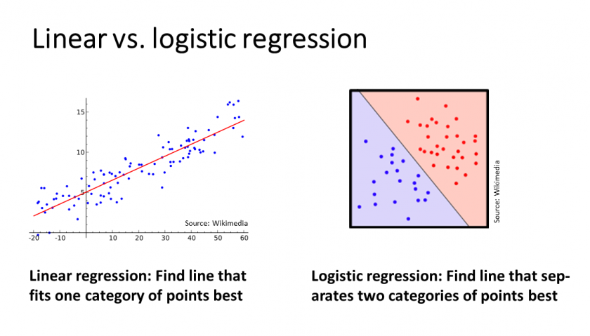
Now, how does a logistic regression work? One hint lies in the name of the glm function: generalized linear model. Whereas with standard linear regression (see e.g., here: Learning Data Science: Modelling Basics) in the 2D-case one tries to find the best-fitting line for all points, with logistic regression you try to find the best line which separates the two classes (in this case pregnant vs. not pregnant):
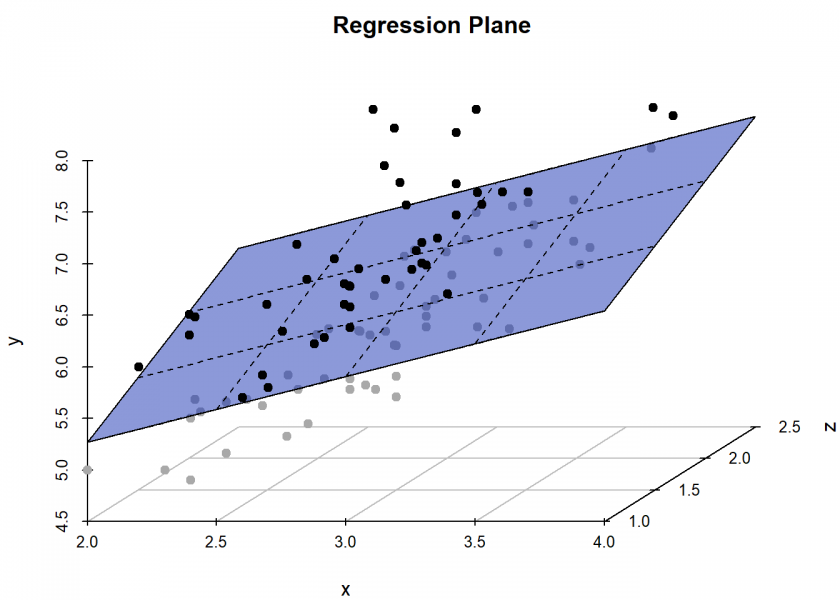
In the n-D-case (i.e. with n features) the line becomes a hyperplane, e.g., in the 3D-case:
One learning from all of that is again that simple models are oftentimes quite good and better interpretable than more complicated models! Another learning is that even with simple models and enough data very revealing (and sometimes embarrassing) information can be inferred… you should keep that in mind too!
UPDATE November 24, 2020
To see that logistic regression is even the core of Neural Networks (a.k.a. Deep Learning) see this post: Logistic Regression as the Smallest Possible Neural Network.
UPDATE December 6, 2022
I created a video for this post (in German):
Interesting article. In a real life situation how to you define the Prediction variable Pregnant in order to build the model?
Thank you, Andrew.
For filling the target variable Pregnant in your training data set you can either employ some strategy to get this information from your customers (e.g. by a survey) or you can try to infer it, e.g. by identifying customers who from a certain point in time on buy diapers on a regular basis.